PPO to GRPO
A complete derivation from policy gradient to GAE, importance sampling, and PPO-Clip, and GRPO
The PPO Algorithm
Let’s start by defining a few concepts as the foundation for everything that follows:
- Action: the set of selectable actions, i.e., the moves the model can take next.
- Policy: a policy function that takes a state as input and outputs a probability distribution over actions, usually denoted by $\pi$, e.g. $\pi(action1|S_t)=0.78\dots$
- Trajectory: denoted by $\tau$, a sequence of states and actions, where $S_{t+1}=f(S_t,a_t)$ is deterministic, or $S_{t+1}=f(*|S_t,a_t)$ is stochastic.
- Return: the cumulative sum of rewards from the current time step until the end.
Expectation:
$$E(x)_{x \sim p(x)} = \sum_{x} x * p(x) \approx \frac{1}{n} \sum_{i=1}^{n} x_i \quad (x_i \sim p(x))$$Goal 1: train a policy network $\pi$ that, in every state $S$, outputs actions such that the expected Return is maximized. Goal 2: train a policy network $\pi$ that maximizes the expected Return over all trajectories.
Policy Gradient
Let $R(\tau)$ be the total return obtained by trajectory $\tau$. Under the current policy, the expected return over all possible trajectories is:
$$E(R(\tau))_{\tau \sim P_\theta(\tau)} = \sum_{\tau} R(\tau)P_\theta(\tau)$$$$\nabla E(R(\tau))_{\tau \sim P_\theta(\tau)} = \nabla \sum_{\tau} R(\tau)P_\theta(\tau)$$$$= \sum_{\tau} R(\tau)\nabla P_\theta(\tau)$$$$= \sum_{\tau} R(\tau)\nabla P_\theta(\tau)\frac{P_\theta(\tau)}{P_\theta(\tau)}$$$$= {\color{#4285F4}{\sum_{\tau} P_\theta(\tau)} R(\tau)}\frac{\nabla P_\theta(\tau)}{P_\theta(\tau)}$$$$\approx \frac{1}{N} \sum_{n=1}^N R(\tau^n) \frac{\nabla P_\theta(\tau^n)}{P_\theta(\tau^n)}$$$$= \frac{1}{N} \sum_{n=1}^N R(\tau^n)\nabla \log P_\theta(\tau^n)$$The last step uses $\nabla \log f(x) = \frac{\nabla f(x)}{f(x)}$.
A state is fully determined by the previous state and action, so the probability of a trajectory is the product of all its states and the actions taken in each state:
$$= \frac{1}{N} \sum_{n=1}^N R(\tau^n)\nabla \log \prod_{t=1}^{T_n} P_\theta(a_n^t|s_n^t)$$$$= \frac{1}{N} \sum_{n=1}^N R(\tau^n) \sum_{t=1}^{T_n} \nabla \log P_\theta(a_n^t|s_n^t)$$$$= \frac{1}{N} \sum_{n=1}^N \sum_{t=1}^{T_n} R(\tau^n)\nabla \log P_\theta(a_n^t|s_n^t)$$Dropping the gradient symbol, the objective for gradient ascent is $\frac{1}{N} \sum_{n=1}^N \sum_{t=1}^{T_n} R(\tau^n)\log P_\theta(a_n^t|s_n^t)$. When we perform the gradient update, the loss is defined as:
$$\text{Loss} = -\frac{1}{N} \sum_{n=1}^N \sum_{t=1}^{T_n} \color{#4285F4}{R(\tau^n)} \log \color{#EA4335}{P_\theta(a_n^t|s_n^t)}$$This means we need to collect the $R(\tau^n)$ produced by every trajectory. Collecting data this way is very slow, consumes a lot of GPU/CPU memory, and has a deeper problem:
$$\frac{1}{N} \sum_{n=1}^N \sum_{t=1}^{T_n} {\color{#4285F4}R(\tau^n)}\nabla \log P_\theta(a_n^t|s_n^t)$$The problem: $R(\tau^n)$ is the total score of the entire game. But in reality, an action $a_t$ taken at time $t$ cannot influence anything that happened before time $t$. Using the total score to evaluate the current action is unreasonable.
$$R(\tau^n) \rightarrow \sum_{t'=t}^{T_n} \gamma^{t'-t} r_{t'}^n = \color{#4285F4}{R_t^n}$$We replace the total return with the future cumulative return $R_t^n$, measured from the current time $t$ until the end of the game. A discount factor $\gamma$ (Gamma, between 0 and 1) is usually introduced here: the more distant a reward, the less reference value it carries. $r_{t'}^n$ denotes the immediate reward of a specific step. The update becomes:
$$\frac{1}{N} \sum_{n=1}^N \sum_{t=1}^{T_n} \color{#4285F4}{R_t^n} \nabla \log P_\theta(a_n^t|s_n^t)$$But a problem remains: what if every reward in an environment is positive, or every reward is negative? If everything is “bad”, the model would keep updating downward forever. So we should introduce a baseline and judge each action against that baseline.
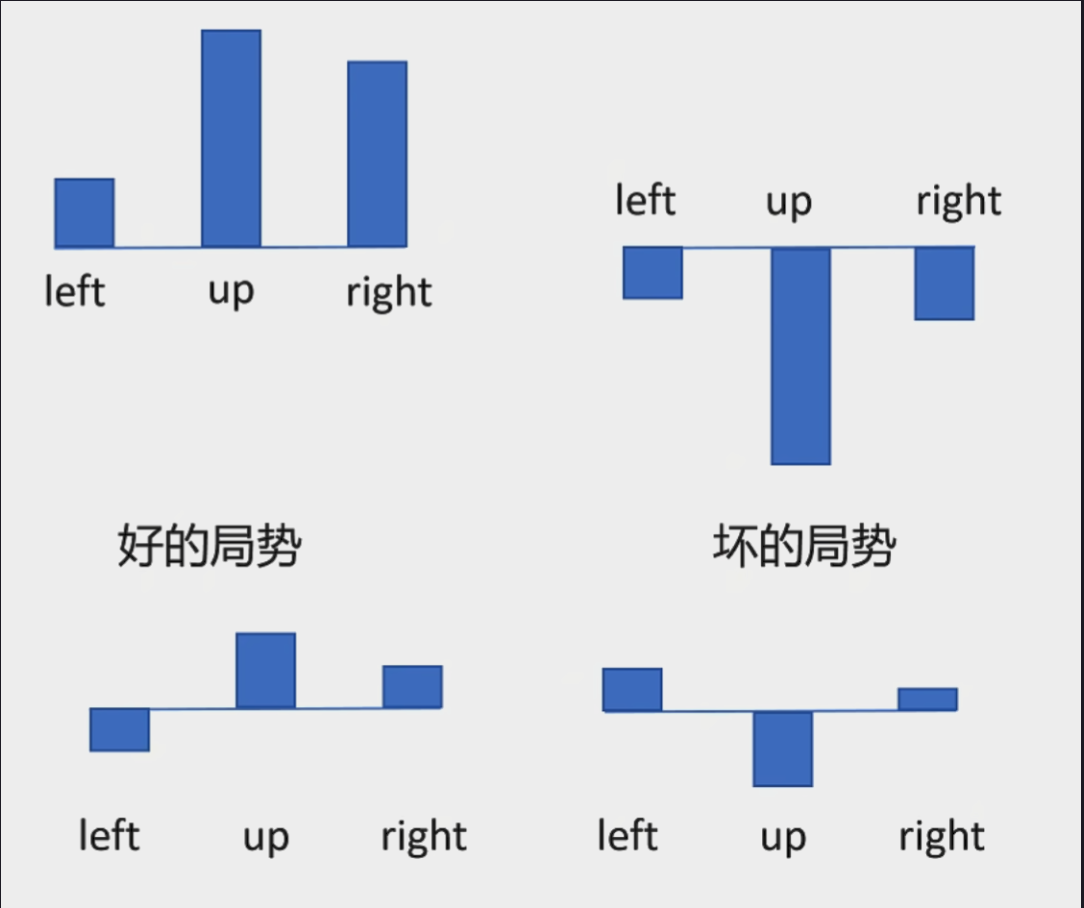
With the baseline in place, we get the following optimized formula:
$$=\frac{1}{N} \sum_{n=1}^N \sum_{t=1}^{T_n} (R_t^n - B(s_n^t)) \nabla \log P_\theta(a_n^t|s_n^t)$$$B(s_n^t)$: the Baseline. It is usually the average expected score of the current state $s_n^t$ (in practice, another neural network — a value network, the Critic — is trained to predict the value $V(s)$ of the state as the baseline).
$(R_t^n - B(s_n^t))$: this difference is called the advantage function (usually denoted $A_t$). It measures: “compared with picking blindly at random in this state (average level), how much better or worse is the action I just took?”
The Advantage Function
Starting from our baseline-corrected formula:
$$\frac{1}{N} \sum_{n=1}^N \sum_{t=1}^{T_n} (R_t^n - B(s_n^t)) \nabla \log P_\theta(a_n^t|s_n^t)$$we introduce a few more definitions:
- Action-Value Function (the $Q$ function): $R_t^n$ is a single random sample each time — high variance, unstable training. $Q_\theta(s, a)$ is the expected return when taking action a in state s.
- State-Value Function (the $V$ function): $V_\theta(s)$ is the expected return in state s.
- Advantage Function (the $A$ function): $A_\theta(s, a) = Q_\theta(s, a) - V_\theta(s)$ — how much advantage taking Action a in state s brings compared with other actions.
So we can replace the sample-based $(R_t^n - B(s_n^t))$ with the expectation $A_\theta(s, a)$, and the formula becomes:
$$\frac{1}{N} \sum_{n=1}^N \sum_{t=1}^{T_n} A_\theta(s_n^t, a_n^t) \nabla \log P_\theta(a_n^t|s_n^t)$$When computing the advantage function, we can look k steps ahead and use the actual rewards:
- One-step estimate: $A_\theta^1(s_t, a) = r_t + \gamma * V_\theta(s_{t+1}) - V_\theta(s_t)$
- Two-step estimate: $A_\theta^2(s_t, a) = r_t + \gamma * r_{t+1} + \gamma^2 * V_\theta(s_{t+2}) - V_\theta(s_t)$
- Three-step estimate: $A_\theta^3(s_t, a) = r_t + \gamma * r_{t+1} + \gamma^2 * r_{t+2} + \gamma^3 V_\theta(s_{t+3}) - V_\theta(s_t)$
- $T$-step estimate: $A_\theta^T(s_t, a) = r_t + \gamma * r_{t+1} + \gamma^2 * r_{t+2} + \gamma^3 * r_{t+3} + \dots + \gamma^T * r_T - V_\theta(s_t)$
Introducing $\delta_t^V = r_t + \gamma * V_\theta(s_{t+1}) - V_\theta(s_t)$, the advantage estimates can be rewritten as:
$$A_\theta^1(s_t, a) = \delta_t^V$$$$A_\theta^2(s_t, a) = \delta_t^V + \gamma \delta_{t+1}^V$$$$A_\theta^3(s_t, a) = \delta_t^V + \gamma \delta_{t+1}^V + \gamma^2 \delta_{t+2}^V$$$$\vdots$$How many steps ahead should we look when updating the parameters? Looking at fewer steps gives higher bias; looking at more steps gives higher variance. GAE proposes looking at all steps and taking a weighted average:
$$A_\theta^{GAE}(s_t, a) = (1 - \lambda)(A_\theta^1 + \lambda * A_\theta^2 + \lambda^2 * A_\theta^3 + \dots)$$Here $(1 - \lambda)$ is a normalization coefficient. Since the infinite geometric series satisfies $1 + \lambda + \lambda^2 + \dots = \frac{1}{1-\lambda}$, multiplying by $(1-\lambda)$ ensures all the weights sum to exactly 1. Let’s keep simplifying by substituting the $\delta$ expansions into $A^1, A^2 \dots$
$$= (1 - \lambda)(\delta_t^V + \lambda * (\delta_t^V + \gamma \delta_{t+1}^V) + \lambda^2 (\delta_t^V + \gamma \delta_{t+1}^V + \gamma^2 \delta_{t+2}^V) + \dots)$$$$= (1 - \lambda) \big( \delta_t^V(1 + \lambda + \lambda^2 + \dots) + \gamma \delta_{t+1}^V * (\lambda + \lambda^2 + \dots) + \dots \big)$$We know $1+\lambda+\lambda^2+\dots = \frac{1}{1-\lambda}$, and after factoring out $\lambda$, $\lambda+\lambda^2+\dots = \frac{\lambda}{1-\lambda}$. Substituting:
$$= (1 - \lambda) \left( \delta_t^V \frac{1}{1-\lambda} + \gamma \delta_{t+1}^V \frac{\lambda}{1-\lambda} + \dots \right)$$which gives the final result:
$$A^{GAE}(s_t, a) = \sum_{b=0}^{\infty} (\gamma \lambda)^b \delta_{t+b}^V$$Off-Policy and Importance Sampling
Since every update is on-policy — meaning we must collect fresh rewards before each round of training — things are very slow. Instead, we can run a reference model to collect data, then train on that collected data multiple times.
Importance sampling is a mathematical trick that lets us estimate the expectation under distribution $p(x)$ using samples drawn from distribution $q(x)$:
$$\mathbb{E}(f(x))_{x \sim p(x)} = \sum_x f(x) * p(x)$$$$= \sum_x f(x) * p(x) \frac{q(x)}{q(x)}$$$$= \sum_x f(x) \frac{p(x)}{q(x)} * q(x)$$$$= \mathbb{E} \left( f(x)\frac{p(x)}{q(x)} \right)_{x \sim q(x)}$$$$\approx \frac{1}{N} \sum_{n=1}^N f(x)\frac{p(x)}{q(x)} \quad (x \sim q(x))$$$\theta$: the parameters of the current policy network being trained. $\theta'$: the parameters of the old policy network that interacted with the environment and actually collected the data.
Sampling with the new policy $\theta$, the gradient update is:
$$\frac{1}{N} \sum_{n=1}^N \sum_{t=1}^{T_n} A_\theta^{GAE}(s_n^t, a_n^t) \nabla \log P_\theta(a_n^t|s_n^t)$$Now switching to the old policy, or reference policy $\theta'$:
$$= \frac{1}{N} \sum_{n=1}^N \sum_{t=1}^{T_n} A_{\theta'}^{GAE}(s_n^t, a_n^t) \frac{P_\theta(a_n^t|s_n^t)}{P_{\theta'}(a_n^t|s_n^t)} \nabla \log P_\theta(a_n^t|s_n^t)$$$$= \frac{1}{N} \sum_{n=1}^N \sum_{t=1}^{T_n} A_{\theta'}^{GAE}(s_n^t, a_n^t) \frac{P_\theta(a_n^t|s_n^t)}{P_{\theta'}(a_n^t|s_n^t)} \color{#4285F4}{\frac{\nabla P_\theta(a_n^t|s_n^t)}{P_\theta(a_n^t|s_n^t)}}$$$$= \frac{1}{N} \sum_{n=1}^N \sum_{t=1}^{T_n} A_{\theta'}^{GAE}(s_n^t, a_n^t) \frac{\nabla P_\theta(a_n^t|s_n^t)}{P_{\theta'}(a_n^t|s_n^t)}$$$$\text{Loss} = - \frac{1}{N} \sum_{n=1}^N \sum_{t=1}^{T_n} A_{\theta'}^{GAE}(s_n^t, a_n^t) \frac{P_\theta(a_n^t|s_n^t)}{P_{\theta'}(a_n^t|s_n^t)}$$The PPO Strategy
We obtained an objective that can reuse old data through importance sampling, but it has a fatal flaw: if the new policy $\theta$ and the old policy $\theta'$ diverge too much, the importance weight $\frac{P_\theta}{P_{\theta'}}$ explodes and the model collapses outright. To fix this, PPO proposes two ways of limiting the size of policy updates.
TRPO:
$$Loss_{ppo} = - \frac{1}{N} \sum_{n=1}^N \sum_{t=1}^{T_n} A_{\theta'}^{GAE}(s_n^t, a_n^t) \frac{P_\theta(a_n^t|s_n^t)}{P_{\theta'}(a_n^t|s_n^t)} + \beta KL(P_\theta, P_{\theta'})$$- $KL(P_\theta, P_{\theta'})$: the KL divergence, a mathematical tool for measuring how much two probability distributions differ. Here it measures how far apart the action distributions output by the new and old policy networks are.
- $\beta$: the penalty coefficient.
The clipped surrogate objective (PPO-Clip):
For clarity, abbreviate the importance ratio as $r_t(\theta) = \frac{P_\theta(a_n^t|s_n^t)}{P_{\theta'}(a_n^t|s_n^t)}$. The formula becomes:
$$Loss_{ppo2} = - \frac{1}{N} \sum_{n=1}^N \sum_{t=1}^{T_n} \min \left( \color{#EA4335}{A_{\theta'}^{GAE}(s_n^t, a_n^t) \frac{P_\theta(a_n^t|s_n^t)}{P_{\theta'}(a_n^t|s_n^t)}}, \color{#4285F4}{\text{clip}\left(\frac{P_\theta(a_n^t|s_n^t)}{P_{\theta'}(a_n^t|s_n^t)}, 1-\varepsilon, 1+\varepsilon\right) A_{\theta'}^{GAE}(s_n^t, a_n^t)} \right)$$- $\varepsilon$: the clipping hyperparameter, usually 0.2. This means the new policy’s probabilities may be at most $1.2\times$ or $0.8\times$ those of the old policy.
- $\text{clip}(r_t(\theta), 1-\varepsilon, 1+\varepsilon)$: the clipping function. If the ratio $r_t(\theta)$ exceeds $1+\varepsilon$, it is forcibly held at $1+\varepsilon$; if it falls below $1-\varepsilon$, it is forcibly held at $1-\varepsilon$.
Clipping is the mainstream approach in industry today, and it is also simple to implement; the min function here forces the model to make conservative updates, making training more robust.
GRPO
PPO now has a complete path from rewards to policy updates: use a critic to construct advantages, then optimize the clipped objective. GRPO changes the advantage-construction step. When several answers address the same question, their rewards provide a local comparison without a separate value prediction.
In the outcome-reward setting used here, sample $G\geq2$ answers $o_1,\ldots,o_G$ from $\pi_{\mathrm{old}}$ for question $q$. Score the completed answers to obtain $r_1,\ldots,r_G$. Here $G$ is the group size, unlike the earlier return $G_t$; $r_i$ scores an entire answer, unlike a step reward $r_t$.
First compute the group’s mean reward and subtract it from each answer’s reward. This centers the comparison on the question’s sampled answers:
$$ \bar r=\frac1G\sum_{j=1}^G r_j, \qquad \text{centered reward}_i=r_i-\bar r. $$Second, divide by the group’s reward standard deviation to scale the differences. The original GRPO-style advantage used here is:
$$ \sigma_r=\sqrt{\frac1G\sum_{j=1}^G(r_j-\bar r)^2}, \qquad \hat A_i=\frac{r_i-\bar r}{\sigma_r+\varepsilon_{\mathrm{num}}}. $$GRPO uses the same current-versus-old comparison as PPO. For token $t$ in answer $o_i$, the state is the question $q$ followed by the prefix $o_{i, At a fixed prefix $s$, one relevant KL direction is: The complete objective can now be assembled one token at a time. Its reward term uses the same clipped ratio as PPO, with the answer’s group-relative advantage $\hat A_i$. The reference penalty is then subtracted: The original GRPO averaging convention first averages over tokens within each answer, then over answers within the group. Questions $q$ are sampled from the training-question distribution $\mathcal D$. Let $|o_i|$ be the number of generated tokens in answer $i$: Fllowed table provides a schematic comparison of common model configurations:
Policy / Role / When it changes $\pi_\theta$ Generates the probabilities being optimized.。 Changes at each optimization step. $\pi_{\mathrm{old}}$ Generates the current batch and supplies the importance-ratio denominator. Fixed during this batch’s updates; refreshed for later sampling. $\pi_{\mathrm{ref}}$ Supplies the comparison distribution for the KL penalty. Usually fixed throughout training. 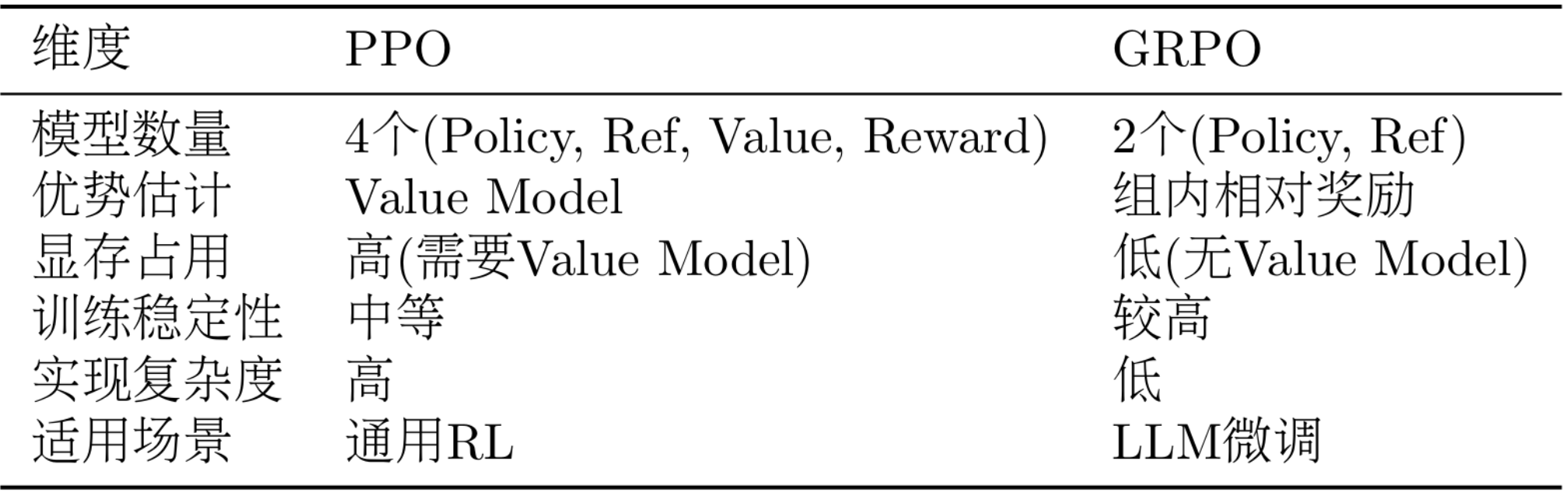
Comments