NOTE:Retrieval-Augmented Generation
Notes and Reflections on the Paper “Retrieval-Augmented Generation”
Overview
Paper link: Retrieval-Augmented Generation
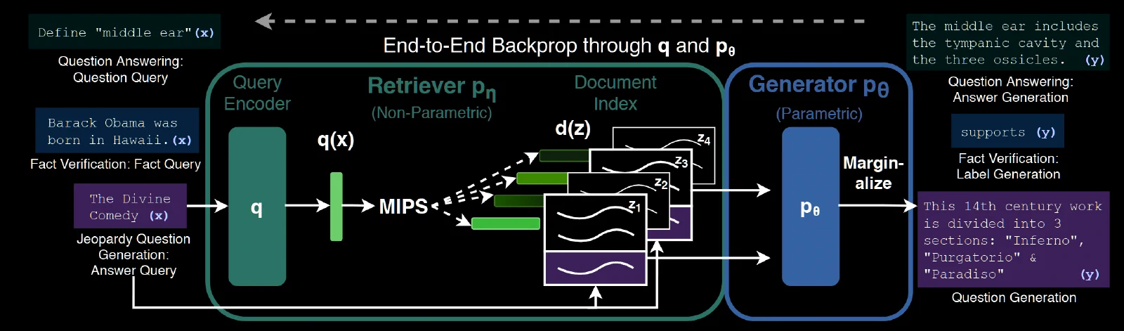
The overall process is as follows: for a specific question, the system first uses MIPS to retrieve relevant documents from the knowledge base, then “passes” them to the large model, which combines that knowledge to produce the final answer.
Questions: the concrete details of the MIPS method; how the documents are passed to the large model (by augmenting the context, by modifying the query, or by making changes at the token level); what marginalization is, and why it is needed.
RAG-Sequence Model and RAG-Token Model
RAG-Sequence: the generated answer relies on only a single document. This model suits cases where the answer is strongly coherent and comes from a single source. When decoding the answer, the model generates a complete candidate answer sequence separately for each document, and at the end evaluates which complete sequence has the highest overall probability.
$$p_{\text{RAG-Sequence}}(y\vert{}x) \approx \sum_{z \in \text{top-k}(p(\cdot\vert{}x))} p_\eta(z\vert{}x) p_\theta(y\vert{}x, z) = \sum_{z \in \text{top-k}(p(\cdot\vert{}x))} p_\eta(z\vert{}x) \prod_{i}^N p_\theta(y_i\vert{}x, z, y_{1:i-1})$$RAG-Token: every time a token is generated, the model consults the different documents again, synthesizing information from multiple sources; this suits answers that need to be pieced together from several sources. The retriever finds the top-$k$ documents. When the generator is about to predict the next word, it computes a next-word probability distribution based on each of the $k$ documents, aggregates them (marginalizes) to settle on that word; when predicting the word after that, it re-examines the $k$ documents and repeats the process.
$$p_{\text{RAG-Token}}(y\vert{}x) \approx \prod_{i}^N \sum_{z \in \text{top-k}(p(\cdot\vert{}x))} p_\eta(z\vert{}x) p_\theta(y_i\vert{}x, z, y_{1:i-1})$$Retriever: DPR
DPR employs a Bi-encoder architecture, whose core working mechanism is as follows:
- Text vectorization:
- Document encoder: A $\text{BERT}_{\text{BASE}}$-based document encoder is used to map each document $z$ to a dense vector representation, denoted as $d(z)$. The formula is expressed as: $d(z) = \text{BERT}_d(z)$.
- Query encoder: Similarly, a $\text{BERT}_{\text{BASE}}$-based query encoder is used to map the user’s input query $x$ to a dense vector representation, denoted as $q(x)$. The formula is: $q(x) = \text{BERT}_q(x)$.
- Similarity Calculation and Probability Distribution: The probability $p_\eta(z\vert{}x)$ of retrieving a particular document is proportional to the exponential of the dot product (inner product) between the query vector and the document vector. Mathematically, this is expressed as: $$p_\eta(z\vert{}x) \propto \exp(d(z)^\top q(x))$$
“Parametric memory” refers to knowledge that the model compresses and stores inside itself through its weights (e.g., the connection weights of a neural network) during training. The parameters of pre-trained models such as BERT or BART are their parametric memory.
“Non-parametric memory” is entirely different. It is like an external knowledge base, or an external hard drive attached to the model; the knowledge is kept outside the model in raw, standalone data form.
MIPS is responsible for quickly finding, among the vast collection of knowledge-base vectors, the top-$k$ vectors with the largest inner product (i.e., the most similar ones) with ${\displaystyle q(x)}$. Computing dot products one by one would be far too slow, and MIPS exists precisely to do this quickly. In the paper, the concrete implementation uses the FAISS library combined with the HNSW algorithm.
RAG’s Fine-tuning Process (Overall Workflow)
Forward:
- The user inputs a question $x$.
- $\text{BERT}_q$ turns it into a vector $q(x)$.
- $q(x)$ is used to run inner-product search (MIPS) over the frozen document store, retrieving the Top-K documents $z$ and their retrieval probabilities $p(z\vert{}x)$.
- The generator BART concatenates the question $x$ with a document $z$ as input and generates the answer word by word, yielding the generation probability $p(y_i\vert{}x, z, y_{\lt i})$.
- The retrieval probability and the generation probability are combined (marginalized) to compute the final value of the loss function (i.e., the negative marginal log-likelihood above).
Backward and Fine-tuning:
- BART: gradients flow back into BART’s encoder (understanding question + document) and decoder (generating the answer). The weight matrices of BART’s internal Self-Attention, Cross-Attention, and FFN layers are updated. Through this, BART learns how to better extract knowledge from the concatenated text and organize it into fluent sentences.
- $\text{BERT}_q$: gradients pass through the generator, flow back to the retrieval probability $p(z\vert{}x)$, then follow the inner-product formula $\exp(d(z)^\top q(x))$ down to the query vector $q(x)$, and continue all the way back into $\text{BERT}_q$’s internal parameters. The attention mechanisms and weights inside $\text{BERT}_q$ are updated accordingly. This way, the next time a similar question is encountered, the vector coordinates output by $\text{BERT}_q$ shift slightly, moving closer to the fixed vectors of those documents that “truly help generate the answer.”
Marginalization and Its Role
Marginalization from the Mathematical Perspective
From two angles — the underlying formulas of probability theory, and backpropagation in deep learning (the direction of gradient flow) — this section explains the elegant design of “marginalization” in the RAG model.
Suppose we need the probability of event $Y$ (generating the correct answer), but the process depends on an intermediate hidden system state $Z$ (which document was retrieved), and $Z$ has several mutually exclusive possibilities (the different documents in the collection). Then we can use the law of total probability.
- For any concrete document $z$, the joint probability of “retrieving document $z$ and generating answer $y$ based on $z$” is: $p(y, z\vert{}x) = p(y\vert{}x, z) \cdot p(z\vert{}x)$.
- Because the true answer does not hinge on any one particular document, we must exhaust and sum over all possible intermediate states $Z$. Mathematically, this means integrating over the latent variable $Z$ (summing in the discrete case): $$p(y\vert{}x) = \sum_{z} p(y\vert{}x, z) p(z\vert{}x)$$
- In the RAG model, to keep the computation tractable, the range of the summation is “truncated” from the infinite document space to an approximation over the Top-K documents found by MIPS, i.e., $z \in \text{top-k}(p(\cdot\vert{}x))$.
This is the mathematical form of marginalization. In deep learning, however, its most important significance lies in the gradient backpropagation that follows.
Marginalization from the Gradient Perspective
As mentioned in Section 2.4, RAG has no labels telling the retriever “which document to retrieve”; its objective is to minimize the negative marginal log-likelihood:
$$\mathcal{L} = -\log p(y\vert{}x) = -\log \sum_{z \in \text{Top-K}} p_\theta(y\vert{}x, z) p_\eta(z\vert{}x)$$When we compute the gradient with respect to the retriever’s parameters $\eta$, we obtain:
$$\frac{\partial \mathcal{L}}{\partial \eta} = - \frac{1}{\sum_{z'} p_\theta(y\vert{}x, z') p_\eta(z'\vert{}x)} \sum_{z \in \text{Top-K}} p_\theta(y\vert{}x, z) \frac{\partial p_\eta(z\vert{}x)}{\partial \eta}$$This gradient formula reveals how the model teaches itself to retrieve: if a well-chosen document ${\displaystyle z}$ is selected, then $p_\theta(y\vert{}x, z)$ will be high, and the gradient will push the update in that direction. Through its weighted-sum form, it implicitly converts BART’s success or failure directly into a dynamic evaluation signal.
Experiments and Thinks
The authors split the articles of the December 2018 Wikipedia dump into passages of roughly 100 words each — 21 million passages in total — and treat each passage as one document.
The authors evaluated the two RAG models on four tasks: open-domain QA, abstractive QA, Jeopardy question generation, and fact verification.
Even without using any decoding strategies specifically designed to promote diversity, the generative diversity of RAG models is significantly higher than that of the base BART model. Among them, RAG-Sequence exhibits higher diversity than RAG-Token. This suggests that incorporating external documents as context naturally enriches the vocabulary and expressions used by the model when generating text. In retrieval-intensive scenarios such as open-domain QA, RAG-Seq performs noticeably better, whereas in imprecise scenarios such as generating responses to dangerous edge cases, RAG-Token performs better because it can integrate information from multiple documents.
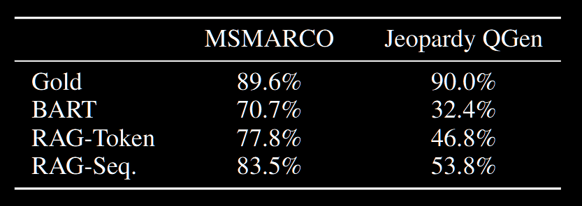
One interesting finding: on Jeopardy question generation, RAG-Token’s generation diversity is actually lower than RAG-Seq’s. Since RAG-Token can piece together information from multiple documents, one would expect its vocabulary and phrasing to be richer and more diverse. The core reason is: “RAG-Token’s token-level fusion is essentially a form of probabilistic smoothing and consensus compromise, whereas RAG-Sequence is a form of path locking and individuality preservation.”
- In RAG-Token, every time the model generates a word, it takes a weighted sum of the probability distributions produced by the $k$ documents. Among these $k$ documents, if document ${\displaystyle A}$ strongly suggests an obscure, advanced word ${\displaystyle w_1}$ while all the other documents choose a conservative word ${\displaystyle w_2}$, document ${\displaystyle A}$’s probability gets diluted, and overall diversity drops.
- In RAG-Sequence, by contrast, the summation happens only after the entire sentence has been generated. This forces the model to dig deep into document A’s distinctive line of thought and characteristic vocabulary, producing one complete sentence with a strong personality of its own.
Comments