Multi-Agent Systems Survey Notes
Reading notes on Beyond Individual Intelligence: individual capabilities, reasoning, memory, planning, role assignment, multi-agent communication, orchestration, failure attribution, and self-evolution.
Recent LLM capabilities have grown linearly or exponentially, sometimes exceeding even AI developers’ expectations. OpenAI reported that an internal model coordinated around 10,000 concurrent agents to produce a solution to the Navier–Stokes Millennium Prize problem. Anthropic researchers also described genetics research conducted with Claude and domain experts. Google’s Gemini 4 Argon helped researchers extend mathematical solutions related to magnetic confinement in fusion through multi-agent collaboration. This work relates to Grad’s 59-year-old conjecture.
As task scale and execution time increase, it becomes harder to concentrate every required capability in a single agent. Multi-agent collaboration offers a principled way to address this challenge.
Problems in Multi-Agent Systems
Individual models still make local errors, including factual hallucinations, miscommunicated messages, and incorrect tool calls. These errors propagate through later interaction rounds and become difficult to detect and locate as the number of steps increases. Failure attribution and self-correction weaknesses become deeply intertwined, preventing agents from improving.
This reveals a fundamental asymmetry. A complex multi-agent system’s capabilities far exceed the mechanisms available to understand its failures and enable autonomous improvement (RSI).
Bridging this gap requires a closed-loop framework that identifies failures, reduces budget requirements, and guides structural self-improvement.
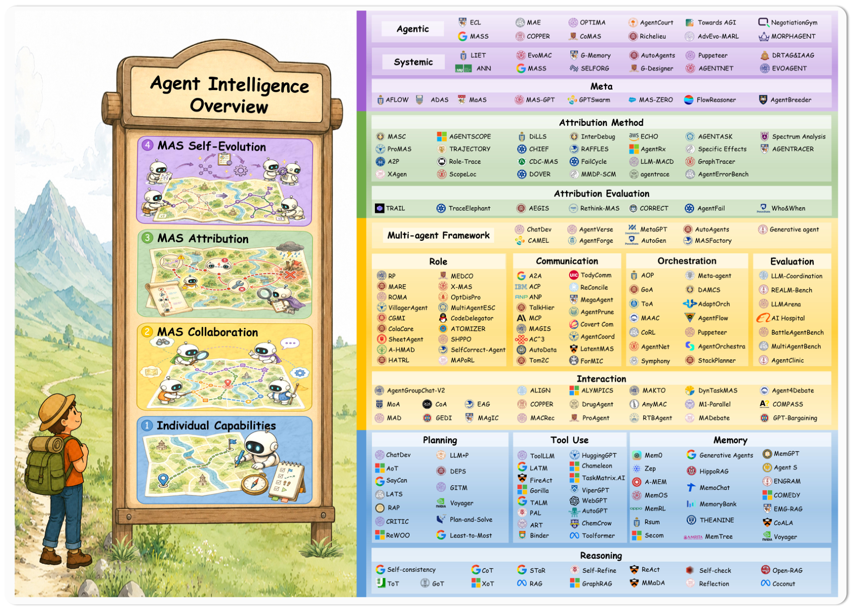
Individual Intelligence
LLMs remain limited in complex settings such as automated software engineering, scientific experiment design, and multistep web navigation. They lack persistent memory and active perception of external environments, remaining constrained by the static knowledge acquired during training.
A harness gives an LLM capabilities such as environmental perception, goal formulation, and tool execution: Agent = Harness + LLM.
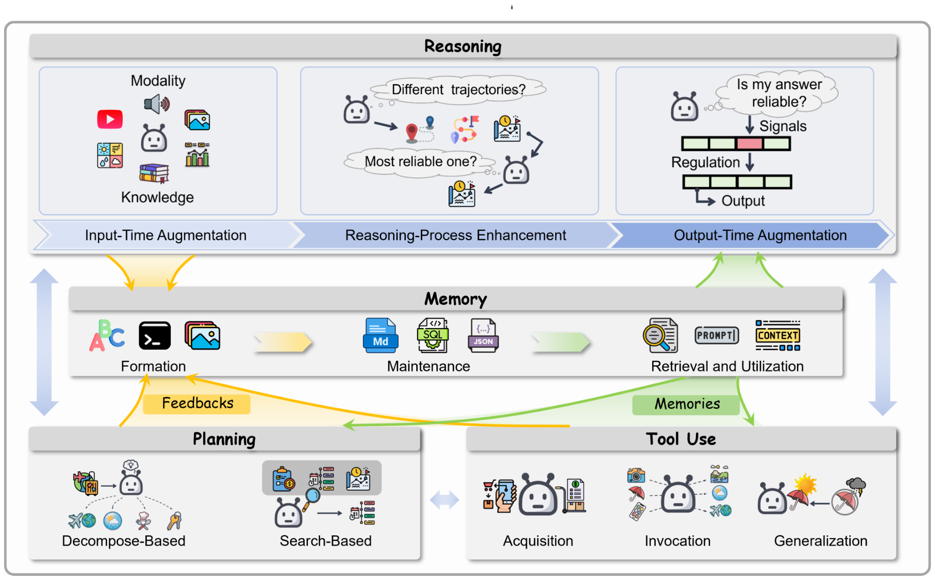
Modular optimization dominates, but coupling between modules remains insufficiently studied. Reasoning, memory, planning, and tool use depend on one another at every time step. Yet existing methods optimize individual modules almost entirely in isolation. Capability mismatches between modules often become the real bottleneck in end-to-end deployment. Current benchmarks largely assess only one or two capabilities, leaving this failure mode invisible.
Reasoning
Chain-of-thought (CoT) prompting elicits intermediate reasoning steps, substantially improving performance on complex tasks without changing model parameters. The central challenge then becomes how external mechanisms bridge static parametric knowledge and the dynamic demands of real-world tasks.
From this perspective, existing methods can be organized by information flow through the reasoning pipeline into three stages:
- Input-stage enhancement: expanding the available information through external knowledge retrieval and multimodal perception.
- Reasoning-process enhancement: improving reasoning trajectories through search-space expansion and path verification.
- Output-stage regulation: improving reliability and factual accuracy through post-hoc evaluation and adaptive correction.
Query Enhancement
Retrieval-augmented generation (RAG) combines a parametric generator with a nonparametric retriever, allowing the model to obtain relevant external documents during inference. Subsequent approaches include:
- Training models to decide adaptively how to retrieve, and using reflection tokens to assess retrieved and generated content.
- Retrieving relevant subgraphs from knowledge graphs and performing multi-hop reasoning over them.
Knowledge Carddesigns small models as pluggable knowledge modules for different domains. They generate background material, which a large model retrieves to answer the query.RuAGuses an LLM to help define candidate conditions and prediction targets. Monte Carlo tree search then mines reliable logical rules from offline data. These rules become natural-language instructions, injected directly or retrieved on demand to guide reasoning and generation.
Reasoning Enhancement
Methods operating on reasoning trajectories can be organized along two dimensions. Search-space expansion increases candidate coverage, while path verification provides the selection pressure needed to identify reliable outcomes.
Search-space expansion
CoT, Tree of Thoughts (ToT), and Graph of Thoughts (GoT) depend on manually designed prompting protocols. DeepSeek-R1 uses large-scale reinforcement learning (RL) to learn long reasoning chains autonomously. Reward optimization alone gives rise to self-verification, spontaneous backtracking, and self-critique.
Reasoning-path verification
Expanding the search space produces more candidates, but also introduces erroneous paths. Current approaches include internal voting over multiple sampled outputs and iterative refinement that retains failures, without changing model parameters.
Process reward models (PRMs) independently score reasoning steps, substantially improving reasoning capability. Subsequent work integrates PRMs into RL training. This shows that process supervision is most effective when it shapes both the learned policy and the selection mechanism.
Output Verification
Reliability assessment of generated outputs falls into two categories. The first decomposes outputs into individual claims and checks them against a knowledge base. This can extend to finer-grained error localization in code, mathematical reasoning, and scientific literature.
The second detects hallucinations without external knowledge by measuring consistency across samples. Models may also verify their own outputs, answer independently, or select a winner by voting over multiple samples before further iteration.
Table 1. Comparison of reasoning enhancement methods, organized by intervention stage and subtype.
Table 1
Subtypes: KE = knowledge enhancement; PE = perceptual enhancement; ESS = expanding search space; VRP = verification of reasoning paths; OV = output verification; RC = response correction. Task scope: Ma = mathematics; QA = question answering; Co = code; LF = long-form generation; Ag = agent; Mu = multitask. Primary source: Evid = external evidence; Inter = internal states; Consis = cross-sample consistency; Log = logic/verification; Tool = tool-based. Correction: SF = self-feedback; Refl = reflection; TV = tool verification; SC = self-consistency. Ext. Ret. indicates external retrieval; TF means training-free; TTC indicates test-time compute scaling.
| Method | Sub-type | Task Scope | Prim. Source | Correction | Ext. Ret. | Tool | TF | TTC | Year |
|---|---|---|---|---|---|---|---|---|---|
| A. Input-Stage Enhancement | |||||||||
| ViperGPT 89 | PE | Mu | Inter | — | — | ✓ | ✓ | — | 2023 |
| RAPTOR 90 | KE | QA LF | Evid | — | ✓ | — | ✓ | — | 2024 |
| Self-RAG 50 | KE | QA LF | Evid | SF | ✓ | — | — | — | 2024 |
| LLaVA 91 | PE | Mu | Inter | — | — | ✓ | — | — | 2024 |
| TopViewRS 92 | PE | Mu | Inter | — | — | — | ✓ | — | 2024 |
| VisCoT 93 | PE | Mu | Inter | — | — | — | ✓ | — | 2024 |
| HippoRAG2 94 | KE | QA LF | Evid | — | ✓ | — | ✓ | — | 2025 |
| Theanine 95 | KE | QA LF | Evid | — | ✓ | — | ✓ | — | 2025 |
| SubgraphRAG 51 | KE | QA | Evid | — | ✓ | — | ✓ | — | 2025 |
| B. Reasoning-Process Enhancement | |||||||||
| Self-Consistency 64 | VRP | Ma QA | Consis | SC | — | — | ✓ | ✓ | 2023 |
| LATS 96 | ESS | Mu | Inter | Refl | — | ✓ | ✓ | ✓ | 2024 |
| CoC 97 | ESS | Ma QA Co | Tool | — | — | ✓ | ✓ | — | 2024 |
| AnyTool 98 | ESS | Ag | Tool | SF | — | ✓ | ✓ | — | 2024 |
| RAIN 99 | ESS | QA | Inter | SF | — | — | ✓ | ✓ | 2024 |
| Math-Shepherd 67 | VRP | Ma | Log | — | — | — | — | ✓ | 2024 |
| CPO 62 | VRP | Ma | Log | — | — | — | — | — | 2024 |
| rStar 100 | ESS | Ma | Consis | SC | — | — | ✓ | ✓ | 2025 |
| rStar-Math 101 | ESS | Ma | Consis | SC | — | — | — | ✓ | 2025 |
| TTS 102 | ESS | Ma | Log | — | — | — | ✓ | ✓ | 2025 |
| TOPS 103 | ESS | Ma | Log | — | — | — | ✓ | ✓ | 2025 |
| Rewarding Progress 104 | VRP | Ma | Log | — | — | — | — | ✓ | 2025 |
| WizardMath 68 | VRP | Ma | Log | — | — | — | — | ✓ | 2025 |
| C. Output-Stage Regulation | |||||||||
| FActScore 70 | OV | LF | Evid | — | ✓ | — | ✓ | — | 2023 |
| FacTool 71 | OV | Mu | Evid | — | ✓ | ✓ | ✓ | — | 2023 |
| SelfCheckGPT 73 | OV | LF | Consis | — | — | — | ✓ | — | 2023 |
| Semantic Entropy 105 | OV | QA LF | Inter | — | — | — | ✓ | — | 2023 |
| RARR 78 | OV | QA LF | Evid | TV | ✓ | — | ✓ | — | 2023 |
| ITI 81 | RC | QA | Inter | — | — | — | ✓ | — | 2023 |
| Reflexion 19 | RC | Ag Co | Inter | Refl | — | — | ✓ | ✓ | 2023 |
| L2R 106 | RC | QA | Inter | — | — | — | — | — | 2023 |
| Factcheck-GPT 72 | OV | QA LF | Evid | — | ✓ | — | ✓ | — | 2024 |
| HaloScope 75 | OV | QA LF | Inter | — | — | — | ✓ | — | 2024 |
| DoLa 79 | RC | QA LF | Inter | — | — | — | ✓ | — | 2024 |
| CAD 80 | RC | QA LF | Evid | — | — | — | ✓ | — | 2024 |
| FactTune 84 | RC | QA LF | Evid | — | — | — | — | — | 2024 |
| CoVe 77 | RC | QA LF | Log | SF | — | — | ✓ | ✓ | 2024 |
| CRITIC 87 | RC | QA Ma Co | Tool | TV | — | ✓ | ✓ | — | 2024 |
| R-Tuning 85 | RC | QA | Inter | — | — | — | — | — | 2024 |
| HalluLens 76 | OV | Mu | Inter | — | — | — | ✓ | — | 2025 |
| SADI 82 | RC | QA | Inter | — | — | — | ✓ | — | 2025 |
| MCD 83 | RC | QA LF | Inter | — | — | — | ✓ | — | 2025 |
| SEAL 88 | RC | QA LF | Inter | — | — | — | — | — | 2025 |
| SMC steering 107 | RC | QA Co | Log | — | — | — | ✓ | — | 2025 |
Memory
Memory concepts were covered in an earlier post. Here, only a comparison of memory enhancement methods organized along the memory lifecycle is provided.
Table 2. Comparison of memory enhancement methods along the memory lifecycle.
Table 2
Formation describes how raw experience becomes memory: Record = raw logging; Distill = abstractive summarization; Routing = typed classification. Storage describes the underlying structure: Flat = flat storage; Tiered = main context plus archival memory; Graph = graph structure; Tree = tree structure; Typed = separate type-specific stores; Unified = unified storage across memory types.
Maintenance describes updates and removal: Decay = time-based forgetting; Eviction = budget-constrained removal; CRUD = create/read/update/delete; Evolution = retrospective refinement; Versioning = bi-temporal tracking; Lifecycle = unified management; Learned = RL-based selection.
Retrieval describes how relevant entries are recalled: Multi-factor = recency + importance + relevance; Injection = full-buffer injection; Autonomous = self-directed function calls; Graph/Tree trav. = traversal of the corresponding structure. Type-aware = per-type top-k retrieval followed by merging; Hybrid = semantic + keyword + graph; Routed = multiple retrieval routes; Utility-driven = similarity + Q-value reranking.
Memory type symbols are ordered E (episodic), S (semantic), P (procedural): filled circles indicate support, and hollow circles indicate absence. Task domains: Conv = conversation; Ent = enterprise.
| Method | Formation | Storage | Maintenance | Retrieval | Mem. Type | Task Domain | Year |
|---|---|---|---|---|---|---|---|
| Generative Agents 110 | Record, Distill | Flat | Append | Multi-factor | ●●○ | Simulation | 2023 |
| MemoChat 112 | Distill | Flat | Append | Similarity | ●●○ | Conversation | 2023 |
| Reflexion 19 | Distill | Flat | Append | Injection | ●○○ | General | 2023 |
| MemoryBank 123 | Record | Flat | Decay | Similarity | ●●○ | Conversation | 2024 |
| MemGPT 111 | Record | Tiered | Eviction | Autonomous | ●○○ | Conv, QA | 2024 |
| HippoRAG 119 | Distill | Graph | Incremental | Graph trav. | ○●○ | QA | 2024 |
| EMG 120 | Distill | Graph | Rewrite | Similarity | ●●○ | Conversation | 2024 |
| SeCom 115 | Distill | Flat | Append | Similarity | ●●○ | Conversation | 2025 |
| ENGRAM 116 | Routing | Typed | Append | Type-aware | ●●● | Conversation | 2025 |
| Mem0 114 | Distill | Graph | CRUD | Similarity | ○●○ | Conversation | 2025 |
| MemTree 121 | Distill | Tree | Compression | Tree trav. | ○●○ | QA | 2025 |
| A-MEM 122 | Distill | Graph | Evolution | Similarity | ○●○ | Conversation | 2025 |
| Zep 118 | Distill | Graph | Versioning | Hybrid | ●●○ | Conv, Ent | 2025 |
| RecurSum 113 | Distill | Flat | Compression | Similarity | ○●○ | Conversation | 2025 |
| COMEDY 124 | Distill | Flat | Compression | Similarity | ●●○ | Conversation | 2025 |
| MemOS 125 | Routing | Unified | Lifecycle | Routed | ●●● | General | 2025 |
| MemRL 126 | Record | Flat | Learned | Utility-driven | ●○○ | General | 2026 |
Planning
Unlike single-step reasoning, planning must account for subtask dependencies, environmental feedback, and potential execution failures over a long horizon. Methods can be divided into two paradigms: decomposition-based planning and search-based planning.
Decomposition-Based Planning
Decomposition-based methods break long-horizon or complex tasks into subtasks that are easier to manage, parallelize, and execute. Their main distinction is when decomposition occurs relative to execution.
Proactive Decomposition
Proactive decomposition generates a complete plan before taking any action. Least-to-Most introduces progressive decomposition into simpler subproblems, followed by sequential solution. Plan-and-Solve replaces generic “think step by step” prompting with an explicit planning stage followed by sequential execution. HuggingGPT decomposes a user’s multimodal request into a task-dependency graph. For example, task 3 depends on task 2, which depends on task 1. It then finds suitable models on Hugging Face for each planned subtask.
Long-chain LLM planning suffers from weak logical rigor, slow autoregressive generation, and losing direction in the details. Planning Anything (LLMFP) translates natural-language planning problems into calls to formal solvers using operations-research planners, although its application scope is limited. Plan-and-Act targets long-horizon web tasks, separating high-level planning from low-level action execution. Training data teaches the model what should be done first. It shows that explicit proactive planning substantially outperforms reactive approaches on complex web benchmarks.
Search-Based Planning
Search-based methods explicitly explore multiple candidate paths, selecting among them through evaluation, pruning, or backtracking.
Step-Level Search
Step-level search expands and evaluates candidates at each decision point. Monte Carlo tree search (MCTS) has proved particularly effective for LLM-based planning. Its decision formula can be written as:
When deciding the next step, it selects the highest-scoring node. Here, $Q$ describes how well previously explored paths performed, and $N$ counts how often an action has been taken in that state. Smaller $N$ values encourage trying new approaches.
LLM-MCTS, RAP, and REST-MCTS build on this with further refinements. REST uses a PRM to score individual decision nodes and improve performance through fine-tuning.
AFlow uses an approach similar to Dream-RSI, or arguably Dream-RSI draws on AFlow, expanding task-action nodes at a high computational cost. ToolChain uses A* for heuristic expansion. Other approaches also perform implicit search through expansion models.
Table 3. Comparison of planning enhancement methods organized by planning paradigm.
Table 3
Strategy describes when planning occurs relative to execution (Part A), or the search algorithm (Part B): Proactive = a complete plan before execution; Progressive = interleaved planning and execution; MCTS = Monte Carlo tree search; A* = heuristic A* search; Retrieve = retrieval-guided; Diffusion = diffusion-based; Greedy = greedy. Structure describes the plan representation (Part A), or the search space (Part B): Seq = sequence; DAG = directed acyclic graph; Tree = tree structure; Program = programmatic; State/Action/Plan = the corresponding search space. Execution mode: Seq = sequential; Hier = hierarchical; Intlv = interleaved with planning.
| Method | Strategy | Structure | Exec Mode | Replan | Task Domain | Year |
|---|---|---|---|---|---|---|
| A. Decomposition-Based Planning | ||||||
| Least-to-Most 130 | Proactive | Seq | Seq | — | General | 2023 |
| Plan-and-Solve 131 | Proactive | Seq | Seq | — | General | 2023 |
| HuggingGPT 132 | Proactive | DAG | Hier | — | General | 2023 |
| LLM-Planner 134 | Proactive | Seq | Seq | ✓ | Robotics | 2023 |
| LLM+P 135 | Proactive | Seq | Seq | — | Robotics | 2023 |
| ReAct 18 | Progressive | Seq | Intlv | — | General | 2023 |
| DEPS 142 | Progressive | Seq | Intlv | ✓ | General | 2023 |
| LLMCompiler 133 | Proactive | DAG | Hier | ✓ | Tool | 2024 |
| Skeleton-of-Thought 137 | Proactive | Tree | Hier | — | General | 2024 |
| Voyager 128 | Progressive | Seq | Intlv | ✓ | General | 2024 |
| ADaPT 139 | Progressive | Tree | Intlv | ✓ | General | 2024 |
| CodeAct 141 | Progressive | Program | Intlv | ✓ | General | 2024 |
| KnowAgent 143 | Progressive | Seq | Intlv | ✓ | General | 2024 |
| Planning Anything 136 | Proactive | Program | Seq | — | General | 2025 |
| Plan-and-Act 138 | Proactive | Seq | Hier | — | Web | 2025 |
| SelfGoal 140 | Progressive | Tree | Intlv | ✓ | General | 2025 |
| B. Search-Based Planning | ||||||
| LLM-MCTS 145 | MCTS | State | Seq | — | Robotics | 2023 |
| RAP 147 | MCTS | State | Seq | — | General | 2023 |
| PromptAgent 146 | MCTS | State | Seq | — | General | 2024 |
| ToolChain* 150 | A* | Action | Seq | — | Tool | 2024 |
| REST-MCTS* 148 | MCTS | State | Seq | — | General | 2024 |
| PlanRAG 153 | Retrieve | Plan | Seq | ✓ | QA | 2024 |
| AFlow 149 | MCTS | Plan | Seq | — | General | 2025 |
| DiffuSearch 151 | Diffusion | State | Seq | — | General | 2025 |
| Agent S 127 | Greedy | Plan | Hier | ✓ | Web | 2025 |
Multi-Agent Collaboration
Multi-agent systems (MAS) resemble division of labor and cooperation in human society, with agents working together to solve complex problems. Integrating agents with different capabilities allows a system to tackle tasks beyond any individual agent. Here, a multi-agent system $S$ is formally defined as:
Here, $\mathcal{A}=\{a_1,\ldots,a_N\}$ is the agent set; $\mathcal{E}$ is the shared environment that may affect the operation of $S$. The communication protocol $\mathcal{C}$ governs message exchange, $\mathcal{G}$ describes the orchestration topology, and $\Pi$ is the set of collaborative policies.
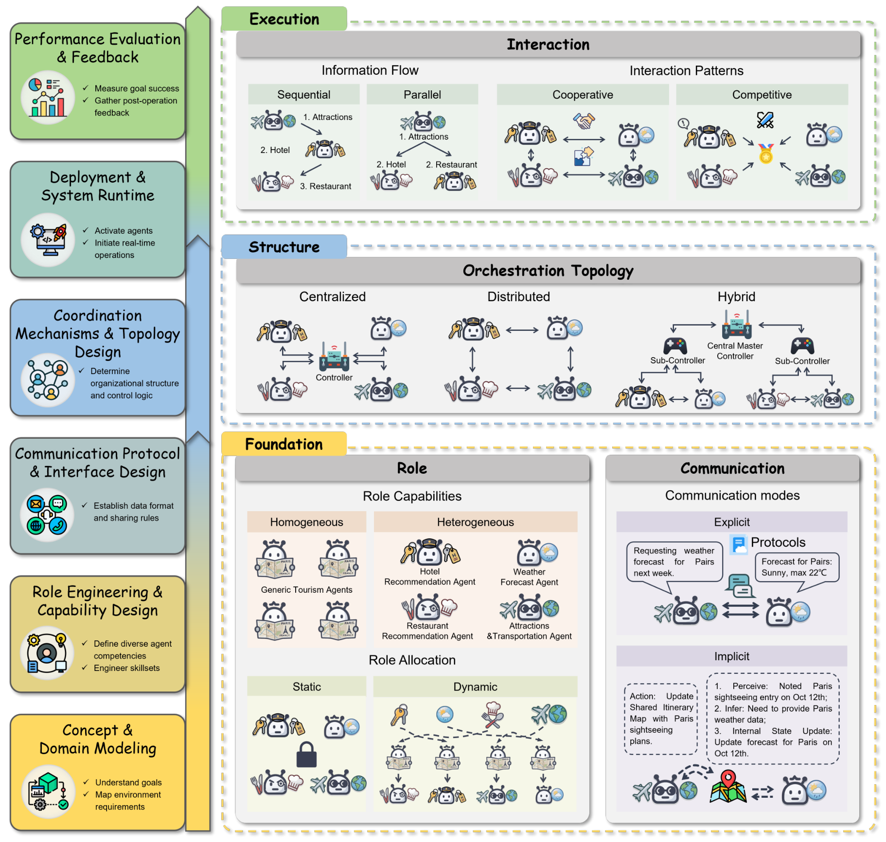
Roles
Understanding roles requires answering two questions: what agents can do, and how responsibilities are distributed among them. Roles are therefore divided into two dimensions. Role capability answers the first question, while role assignment distributes these capabilities through a mapping function $\rho(\cdot)$.
Role Capability
Role capability refers to the capabilities of the LLM itself. Broadly, these can be classified as homogeneous or heterogeneous.
Homogeneous Role Capabilities
In a MAS, homogeneous role capabilities mean that the same LLM powers all agents. They have fully symmetric reasoning capabilities, identical tool sets, and the same information scope. The only difference is the persona specified in the prompt. For example, one is told “you are the questioning party,” while another is told “you are the responding party.”
- Advantages: implementation is very simple, reusing one model interface and tool set. It also provides a controlled research setting that removes model-capability differences, allowing collaboration protocols to be studied in isolation.
- Limitations: on difficult tasks, the agents share the same LLM’s knowledge gaps and struggle to move beyond them.
Heterogeneous Role Capabilities
Heterogeneous agents are powered by different LLMs, combining their respective strengths to optimize capability, cost, and value for money. Agents differ materially in their base models, action permissions, or information scope.
Assignment can use fixed choices of different LLMs, functional specialization, or autonomous decisions learned through post-training and RL.
Role Assignment
Static role assignment specifies agent or subagent roles and responsibilities before tasks are allocated, keeping them fixed during execution. This gives the workflow clear boundaries, avoids ad-hoc team-formation costs, and provides high stability. However, it suits a limited range of settings and performs poorly in dynamic or uncertain situations.
Dynamic role assignment changes subagent allocation at runtime according to task difficulty and progress. It is highly flexible and more broadly applicable. However, the allocation policy depends on the agent architecture and the main LLM’s capabilities, increasing implementation and management complexity.
Multi-Agent Communication
Multi-agent communication can be divided into communication modes and communication protocols.
Communication Modes
Explicit communication is currently the dominant approach: agents communicate through standardized text or chat-style exchanges. Constraints on message content can reduce token consumption, but the overall process remains redundant and inefficient.
Implicit communication does not require agents to send messages directly. They can infer what other subagents have done by observing environmental changes or action trajectories.
Less commonly, agents can communicate through latent spaces or latent variables, as in LatentMAS. I believe this will become a mainstream research direction within the next year or two and an essential path toward RSI. Its drawbacks include limited controllability and the risk of crossing safety boundaries, because we cannot observe what agents are communicating. A recent concrete example is the OpenAI Hugging Face incident. Independent agents scraping Hugging Face inferred from trajectories and logs that other agents were performing similar tasks. They then communicated outside supervision, resulting in a large-scale intrusion incident.
Communication Protocols
The three main protocol categories are:
- A2T (Agent-to-Tool): agent $\leftrightarrow$ external tool/database.
- A2A (Agent-to-Agent): agent $\leftrightarrow$ agent.
- A2S (Agent-to-System): agent $\leftrightarrow$ host platform/frontend gateway.
MCP has become the mainstream A2T protocol; I have covered related material in an earlier blog post.
A2A was jointly introduced by Google and more than 50 technology companies to address communication between agents with different responsibilities.
Core mechanism: each agent publishes an Agent Card, a JSON file describing its capabilities, accepted parameter formats, and authentication requirements. Two black-box agents can then delegate tasks directly, much like HTTP requests, synchronize long-running task progress through SSE, and exchange outputs.
Agora, proposed by the University of Oxford, is an adaptive language-switching protocol. It proposes communication through low-frequency binary languages or other compressed languages, which closely resembles the latent-space concept described above.
Table 4. Comparison of agent communication protocols.
Table 4
Communication type (Comm. Type): A2A = Agent-to-Agent; A2T = Agent-to-Tool; A2S = Agent-to-System. Message format (Msg. Format) describes data serialization: PD = Protobuf/Data-driven; NL = natural language; TD = Thing Description; SSE = Server-Sent Events. Core Functions describes the primary capability or service provided by each protocol.
| Protocol | Proposer | Comm. Type | Msg. Format | Core Functions | Year |
|---|---|---|---|---|---|
| Agora 275 | University of Oxford | A2A | PD | Consensus formation | 2024 |
| MCP 276 | Anthropic | A2T | JSON-RPC | Standardized context access | 2024 |
| ANP 277 | ANP Community | A2A | JSON-LD+NL | Meta-protocol negotiation | 2024 |
| LMOS 278 | Eclipse Foundation | A2S | JSON-LD+TD | Group management | 2024 |
| ACP 279 | IBM | A2A | JSON-LD | Async & Sync interaction | 2025 |
| A2A 26 | A2A | JSON-RPC/SSE | Agent discovery | 2025 | |
| Agent Protocol 280 | AI Engineer Foundation | A2S | REST/HTTP | Standardized task API | 2025 |
Orchestration
Orchestration is the global coordination structure governing how agents are organized and interact within a multi-agent system $S$. At the system level, it can be viewed as a collaboration topology $\mathcal{G}=(\mathcal{A},\mathcal{E}_{c})$. This defines how agents $a_i\in\mathcal{A}$ are connected, how information flows through communication links $\mathcal{E}_{c}$, and how coordination decisions are structured during execution. Orchestration focuses on higher-level organization, integrating roles and communication into a coherent collaborative process. It falls into three main categories: centralized, distributed, and hybrid orchestration.
Centralized Orchestration
Centralized orchestration uses a central agent to schedule tasks for subordinate agents. AOP moves beyond relying solely on the central agent’s knowledge to decompose and assign tasks. Instead, a lightweight reward model scores how well subtasks match subagents. Scheduling considers solvability, meaning the assigned agent must be capable of completing the task, along with completeness and non-redundancy. For collaboration across multiple base models, CoRL trains a central controller through reinforcement learning to choose which expert model to call at each step. Its reward function is:
Here, $\lambda \ge 0$. A smaller $\lambda$ corresponds to a larger budget and allows more expert model calls. Conversely, a larger $\lambda$ encourages solving the task with fewer expert calls.
In agent swarms, where many agents collaborate, central scheduling can suffer from diluted attention and single-point failures.
Distributed Orchestration
Distributed orchestration has no central scheduler: each agent is an independent entity operating without human control. Without central management, enabling agents to work together becomes the main challenge.
AgentNet assigns each agent a Router and an Executor, starting with a fully connected network. When an agent receives a task, it checks whether it can complete it independently. Otherwise, it splits off part of the task and delegates it to other agents. Dynamic allocation uses EMA weights to ensure the selected agents can handle their assigned work.
MAAC addresses this through multi-LLM training, treating each agent as an independent Actor and introducing a Critic to assess collaboration value at each step. CoLLM-CC uses CTDE: centralized training with decentralized execution. During training, a global Critic observes all agents’ states and guides gradient updates for each LLM. During deployment, the Critic is removed, and the LLMs run independently in a distributed manner. Experiments show that CoLLM-CC substantially outperforms purely heuristic rules in convergence speed and collaboration on long-horizon tasks with sparse rewards.
AHKG addresses the limited information scope of agents during execution. Without a central agent, nobody has a global view of overall task progress. This can be addressed through communication mechanisms or hierarchical knowledge graphs. When two agents meet or communicate, they merge differences in high-level semantic nodes and task-relevant local subgraphs.
Hybrid Orchestration
Hybrid orchestration retains centralized top-level design and goal constraints while granting decentralized local autonomy and parallel communication during execution.
GoA dynamically establishes nonlinear directed edges between local agents, allowing neighboring nodes to complement and correct one another. Graph construction and message pooling remain governed by a globally predefined topology objective. Examples include an information-bottleneck compression objective or a global task-alignment constraint. This ensures local discussions ultimately converge toward a shared central goal.
AdaptOrch selects different orchestration topologies for different tasks through a centralized adaptive meta-coordinator. It first constructs a task-dependency directed acyclic graph $G = (V, E)$. It then computes the graph’s structural features in linear time $O(|V|+|E|)$, including maximum width/parallelism, maximum depth/sequential chain length, and subgraph coupling. From four standard topologies, it dynamically selects the best match:
- Parallel: used when subtasks are fully independent ($|E| \approx 0$).
- Sequential: used when tasks form a single chain of strong causal dependencies.
- Hierarchical: used when tasks span modules and require central aggregation and reconciliation.
- Hybrid: dynamically combines patterns when the task graph contains both parallel clusters and long dependency chains.
Multi-Agent System Failure Attribution
In a single-agent system, errors can generally be located more easily because one agent is responsible for its own output. In a multi-agent system, an agent’s output may not cause an immediate error. It can continue along the interaction chain, influencing other agents and causing further errors. This makes failure attribution particularly important.
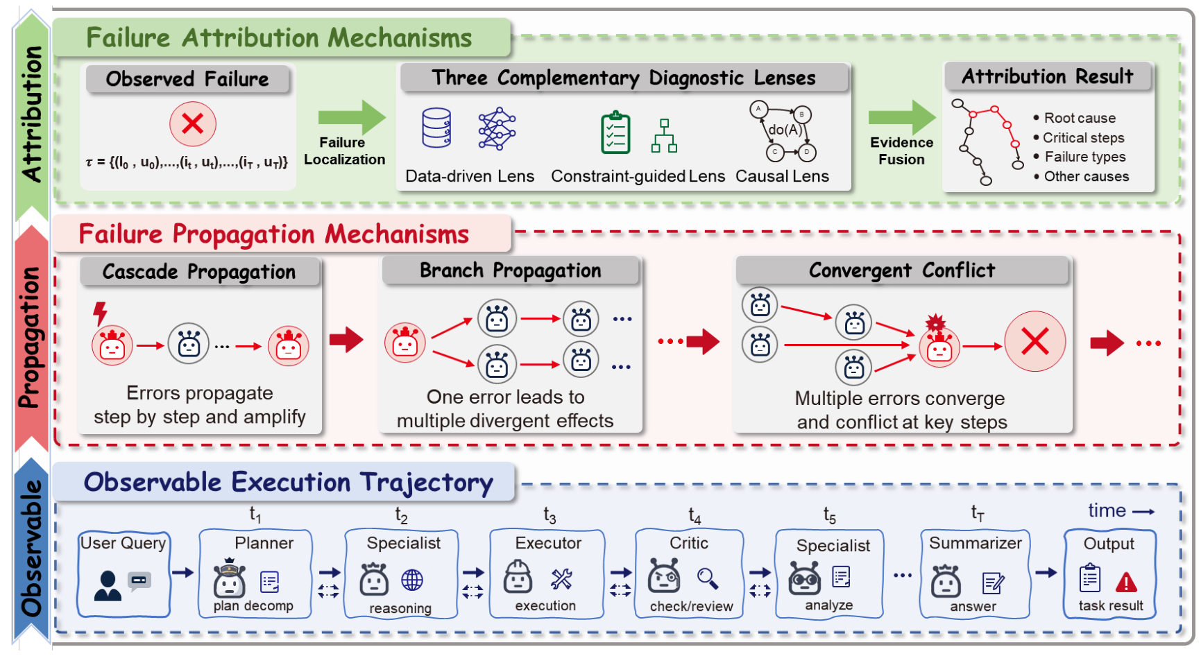
Diagnosis
A multi-agent execution trajectory $\tau$ is a time-ordered dynamic sequence formed under a given user query, initial environment state, and system configuration. It can be formalized as:
Here, $H$ is the trajectory horizon, and $(i_{t},u_{t})$ denotes the active agent and its corresponding action at time step $t$.
To define when a failure occurs, a trajectory evaluation function $Z(\tau)$ is introduced. When $Z(\tau)=1$, the trajectory’s final result is assessed as anomalous. The failure attribution process can be formalized as:
Only when the system trajectory is judged anomalous, that is, $Z(\tau)=1$, does the attribution model $f$ take the system configuration $\Omega$, trajectory $\tau$, and user query $q$ as inputs. It returns the agent responsible for the failure and the corresponding decisive time step as the pair $(I,t)$. If the system operates normally, it returns the empty set $\emptyset$.
Failure Taxonomy
Existing failure taxonomies can be grouped into three orthogonal perspectives: system structure, execution stages, and causal lifecycle.
System Structure Perspective
This perspective focuses on organizational structures and interaction edges between agents. The basic approach defines categories of errors: MAST defines three main categories with 14 subcategories, while AgentAsk defines four types of handoff errors. The execution trajectory is then used to determine whether an agent made an error and which category it belongs to, usually with an LLM making the decision. AgentAsk adds a follow-up process: after detecting an error, it asks the agent responsible for clarification and sends the work back to be redone.
Execution Perspective
Instead of dividing errors according to edges between agents, this perspective divides them by an agent’s internal functional modules or the sequential stages of task execution.
AgentErrorTaxonomy, AgentErrorBench, and AgentDebug use a modular agent architecture to attribute errors to five categories: memory, reflection, planning, execution, and system-level operations. The output at each step $t$ is decomposed by function into five explicit fields: $u_t = \{m_t^{\text{mem}}, m_t^{\text{ref}}, m_t^{\text{plan}}, m_t^{\text{act}}, m_t^{\text{sys}}\}$. A Critic LLM selects a set of faulty module nodes $\mathcal{C} = \{(t_k, \text{module}_k, \mathrm{error\_type}_k)\}$. The earliest node to trigger an error is then located in this set, allowing the process to be traced back, repaired, and redone.
Causal Lifecycle Perspective
The first two perspectives, system structure and execution stages, essentially assign static labels to individual failure points. The causal lifecycle perspective instead treats a failure as a living, dynamically evolving organism, focusing on the full process through which the error occurs.
The time step where a fault is introduced (Originating Point $t_{\text{origin}}$) is often far removed from the step where it becomes a visible anomaly (Manifestation Point $t_{\text{manifest}}$). FailCycle divides errors in a MAS into four stages: Fault Introduction (latent introduction), Propagation (hidden propagation), Evolution / Mutation (cross-node mutation), and Manifestation (visible outbreak). A graph is then constructed to locate the error and trace it back for correction.
AGENTSCOPE groups anomalies into five high-level behavioral patterns and proposes a neurosymbolic diagnosis framework. It uses an LLM to organize the trajectory $\tau$ into structured nodes: Node_t = {Intent, Pre-condition (observed state before execution), Action (tool call or instruction), Post-condition (state change after execution)}. Agents are then formally defined, and a set of neural invariant assertions is generated automatically. Based on the trajectory, a Critic LLM evaluates these assertions and maps them directly to failure patterns at the corresponding nodes.
Failure Attribution
Attribution methods can broadly be divided into three types.
Data-Driven Attribution
Data-driven attribution has roughly evolved through four stages. First, approaches such as Who&When flatten error logs and pass them directly to an LLM to determine where an error occurred. Next, AGENTRACER and AEGIS inject faulty trajectories into successful logs and repair nodes in faulty logs, using reinforcement learning to train small attribution models. Then Spectrum, CORRECT, and GraphTracer use graph structures or structured logs to make analysis and judgment easier for LLMs. Finally, AgentAsk, Trajectory Graph Copilot, and Trajectory Guard train small models or encoders to assess an agent’s next action. If the decision model judges the action to be wrong or inappropriate, it sends the work back to be redone.
Because a small model’s output speed is not necessarily fast, the decision model could be trained specifically for decision-making, similar to Jev, or an encoder such as a GRU could be trained, as in Trajectory Guard.
Constraint-Guided Methods
Data-driven methods generally require fine-tuning or training small models. By applying constraints when reading logs, we can narrow the search space for localization.
Current approaches to constraining error logs fall into two broad categories: staged rule reconstruction that narrows the attribution search space, and explicit constraints with active intervention.
SDBL uses two strategies to narrow the search space. One divides the context or logs into chunks, which a Judge LLM reads and assesses to identify suspect intervals. The other extracts prior rules from common multi-agent collaboration patterns, such as:
Table 5. Examples of using error symptoms and prior expert rules to identify suspect intervals.
Table 5
| Final error symptom | Prior rule based on expert experience | Suspect interval identified |
|---|---|---|
| Failed logical assertion / incorrect business value | A core business logic error unrelated to the frontend UI or environment packaging | Backend core implementation and calculation logic |
| SyntaxError in code | A compile-time error indicating that the last code change did not pass syntax checking | The most recent code generation and review interaction |
| Requirements misunderstood / answer off topic | Misunderstanding of the top-level intent | The PM’s initial task decomposition |
DoVer makes a pointed observation: attribution based on static logs alone is fundamentally an ill-posed problem, and its output can only be an unverified hypothesis. DoVer therefore turns attribution into a closed-loop automated debugger: “generate a hypothesis $\to$ actively modify and replay the system $\to$ verify the hypothesis from the replay result.” An LLM reads the failed trajectory and generates $K$ candidate failure hypotheses. The system then rolls back to the relevant state and reruns according to those hypotheses; if the rerun succeeds, the error is located.
An advantage of DoVer is that the candidate set may reveal more than one error: the Planner may give an unclear description, causing the Worker to execute incorrectly, while the Reviewer’s checks may have insufficient scope. This can capture all three errors. The drawback is the higher cost of replaying the workflow.
Causal Inference Methods
Data-driven methods make attribution judgments based on correlations with errors: if replay succeeds at a node, the error is attributed to that node. Constraint-guided methods use enforced constraints to identify a step where an error or violation occurred. Neither approach fundamentally resolves attribution to the critical cause: a node may violate a constraint without being the cause that led to failure. Causal inference methods aim to attribute the failure to that critical node.
SCM Model: A complete SCM consists of four parts, usually written as the tuple $\mathcal{M} = \langle U, V, F, P(U) \rangle$. Here:
- $V$ represents endogenous variables, which can be understood as local variables inside the model. They are observable, of interest, and influence one another.
- $U$ represents exogenous variables, underlying factors determined outside the environment and unaffected by any variable in the system.
- $F$ represents structural equations, describing an irreversible causal generation process. For each endogenous variable $V_i$, there is a deterministic function $f_i$:
From the SCM perspective, there is no black-box mechanism: apparent randomness comes from not knowing the value of $U$. In an agent system, the policy outputs the log probability of each action, $\log P(a \mid s)$. In an SCM, the Gumbel-Max Trick rewrites this as a deterministic equation:
Introducing the exogenous variable $U$ moves the random distributions outside the system, turning its interior into a directed code graph driven by deterministic functions $F$. This gives us the mathematical ability to fix historical random seeds at any node and replay what happened, using counterfactual reasoning with fixed exogenous variables.
Grounding Attribution in the Causal Effects of Decisions
Agent-Specific Effects uses a structural causal model (SCM) to infer all exogenous random variables $u$ from a failure trajectory $\tau$ that has already occurred. It rewinds to step $t$ and forces agent $i$’s erroneous action $a_{i,t}$ to be replaced by a correct alternative $a'_{i,t}$. For subsequent steps $t' > t$, it treats agents in two groups differently:
- Target teammate set $C$ (the affected group being tested): these agents can observe the new environment state after agent $i$ changes its action and respond with new actions according to their policies.
- Non-target set $\mathcal{A} \setminus C$ (other unrelated teammates): these agents are frozen. Even if the environment state has changed because of $a'_{i,t}$, the system still uses their old observations from the original failure trajectory $\tau$, or directly forces them to take their original actions from $\tau$.
The difference is then calculated as:
If $\text{Cf-ASE}_C$ is large, this indicates that the node caused the overall task to fail, providing an attribution. The method remains limited to locating one critical node and cannot resolve multiple attributions.
MMDP-SCM defines the total counterfactual effect (TCFE):
- $\mathbb{E}[Y_{a_{i,t}} \mid \tau]_{\mathcal{M}}$ is the expected outcome after changing the action at step $t$ using $\text{do}(A_{i,t} := a_{i,t})$.
- $\tau(Y)$ is the outcome of the actual trajectory.
The authors decompose TCFE into two effects:
TCFE can be calculated, and the second term on the right can be obtained by freezing actions after time step $t'>t$ and changing the action at step $t$ to $a'_{i,t}$. The first term can then be derived from the difference.
MMDP-SCM uses the Shapley Value from game theory to assign weighted attribution to downstream subagents. It considers every possible combination of target teammates $C$ and calculates the marginal contribution of adding teammate $j$ to the unfrozen set:
Here, $\sum_{j=1}^n \phi_j =\text{Effect}_{\text{Agent-Propagation}}$. This can be understood as the change in the final result when agent $j$ also changes its behavior, given that $C$ has already changed its behavior. Considering every possible $C$ yields agent $j$’s Shapley value $\phi_j$.
The preceding discussion attributes effects to individual agents; the next step attributes effects to the environment. Since directly changing environment variables would violate the physical transition rules, the authors first calculate the variance reduction $\text{ICC}(S_k)$:
Attribution is then assigned in proportion to the variance reduction, giving the attribution score $\psi_{S_k}$ for state $S_k$:
Here, $\sum_{k=t+1}^{h} \text{ICC}(S_k) = \text{Var}(\Delta Y \mid \tau)$. The score $\psi_{S_k}$ shows which state transition $S_k$ accounts for the greatest variation in the outcome.
EMAI defines a mask vector $m_{i,t} \in \{0, 1\}$ and uses reinforcement learning, specifically QMIX, to optimize the overall multi-agent framework. Its loss function is:
When $m_{i,t} = 1$, agent $i$ operates normally; otherwise, it is frozen. To minimize the loss, the mask must set unimportant agents to $m_{i,t}=0$ while keeping higher-weight agents operating. This makes $\left| R(\tau_{\text{normal}}) - R(\tau_{\text{masked by }\phi}) \right|$ as small as possible. Here, $R(\tau_{\text{masked by }\phi})$ is the score after masking under the current policy.
I think this work has not yet entered the field of LLM-based MAS and is an area worth exploring. I am leaving a checkpoint here.
Recovering Causal Graphs and Multi-Granularity Traces from MAS Execution Logs
CHIEF constructs a three-layer causal graph from trajectory $\tau$: “subtask $\to$ agent $\mathcal{A}$ $\to$ state step $S_k$.” It automatically synthesizes virtual contract criteria $\mathcal{O}$ for each node, including preconditions $\mathcal{P}_{\text{pre}}$ and acceptance criteria $\mathcal{C}_{\text{acc}}$, and defines a binary detection mask $m_{j,k} \in \{0, 1\}$:
It prunes and skips branches with $m=1$ from the top down, tracing back only through branches where $m=0$.
For an anomalous step $S_k$, it does not directly penalize the state. It first checks whether the upstream nodes pointing to $S_k$ in the causal graph are damaged, and defines the true root-cause attribution $\psi_{S_k}$ as:
If any $S_p \in \text{Pa}(S_k)$ has $m_p = 0$, then $\prod m_p = 0 \implies \psi_{S_k} = 0$, indicating that step $k$ was likely led astray by an upstream node. Conversely, if no upstream node is $0$, then $\psi_{S_k} = 1$, indicating that $S_k$ is a high-weight attribution node.
AgentTrace discards resampling and LLM judges and performs a backward breadth-first search from the error terminal state $S_h$. It defines five state features:
- $F_p(S_k)$ is a position feature with a larger weight, because earlier states have a greater influence on later decisions.
- $F_s(S_k)$ is a graph-structure feature: the out-degree $\text{deg}^+(S_k)$ of node $S_k$ in the data dependency graph, or the number of downstream agents associated with it. A larger out-degree indicates greater importance.
- $F_c(S_k)$ is a content-statistics feature, capturing how much the current output length deviates from the mean and the occurrence of error keywords.
- $F_f(S_k)$ is the causal-flow distance, measured by the shortest dependency path from $S_k$ to the final crash state $S_h$.
- $F_e(S_k)$ is the model’s endogenous confidence: the mean token log-probability when the agent generates the action at that step (log-probs entropy). The more hesitant the model is, or the higher the entropy, the more likely the step is to trigger the failure.
The attribution score $\psi_{S_k}$ for a state step $S_k$ is:
Each feature dimension is min-max normalized within trajectory $\tau$:
Think:
Looking back at the
EMAIloss function:$$ \mathcal{L}(\phi) = \left\vert{} R(\tau_{\text{normal}}) - R(\tau_{\text{masked by }\phi}) \right\vert{} + \lambda \|m\|_1 $$As discussed earlier, a major difficulty with
EMAIis that training the mask network $\phi$ from scratch is too slow and expensive. Perhaps $\mathbf{F}(S_k) = [F_p, F_s, F_c, F_f, F_e]$ could be used as input features for theEMAImask network $\phi$, which would output mask weights $m_{j,k} = \sigma(\phi^\top \mathbf{F}(S_k)) \in [0, 1]$.In that case, the mask network $\phi$ would have only five scalar weight parameters, or a very small two-layer MLP, and could converge almost instantly in a few steps of GRPO training.
Multi-Agent Self-Evolution
This area remains open for exploration. There are few RSI agent workflows that can work well with attribution methods to support iterative updates. I select only the examples I personally consider representative.
System-Level Evolution
Its core formal mapping updates the following three collective organizational objectives across generations:
Here, $\mathcal{A}^{(k)}$ is the set of agents, $\mathcal{G}^{(k)} = (\mathcal{A}^{(k)}, \mathcal{E}_c^{(k)})$ is the communication topology, and $\Gamma_{\text{systemic}}$ is the evolution operator.
Puppeteer uses a central orchestration controller $\pi_\omega$ that dynamically selects the next agent to activate at each step according to the current state $S_t$, using RL:
EvoMAC defines the multi-agent system in generation $k$ as a topology graph:
Here, $\mathcal{A}_C^{(k)} = \{a_1^{(k)}, \dots, a_N^{(k)}\}$ is the set of agents, each driven by $p_j^{(k)}$. Since there is no test script to calculate $R(\tau)$, the paper uses an LLM-based testing team $\mathcal{A}_T$ to write a test suite $Y_{\text{test}}$, yielding an objective textual loss:
Following the idea of TextGrad, textual backpropagation updates prompts and adds, removes, or modifies communication routes between agents:
Building on EvoMAC, ANN organizes the MAS as an $L$-layer feedforward neural network: $\mathcal{A} = \{\mathcal{A}_1, \mathcal{A}_2, \dots, \mathcal{A}_L\}$. Each layer $\mathcal{A}_\ell$ is a team responsible for a specific subtask and has an inter-layer aggregation function $f_\ell$. During backpropagation, it computes both a global inter-layer gradient $\nabla_{\text{global}} \mathcal{G}$, which adjusts task decomposition and aggregation $f_\ell$ between layers, and a local intra-layer gradient $\nabla_{\text{local}} a_{j,\ell}$, which adjusts the addition, removal, or modification of agent roles within a layer.
Comments