Graduate Entrance Exam Math Notes: Calculus and Linear Algebra
Complete revision notes for calculus and linear algebra.
These notes organize concepts, examples, derivations, and revision reminders by topic, with the original figures. Apply each result under its stated assumptions and the model and data specified by the exercise.
When working on a new problem, recognize its similarity to a previous problem. While solving it, discover gaps in your understanding of this type of problem, its tools, and its methods, or find that your understanding is not deep enough. By solving the new problem, update and refine your previous understanding at the same time.
Limits, Derivatives, and Differentials
Algebraic Transformations, Recurrences, and Product Derivatives
- For the hyperbolic sine function $y=\dfrac{e^x-e^{-x}}{2}$, solve for the inverse as follows: First rewrite it as $2y+e^{-x}=e^x$, multiply both sides by $e^x$, and set $u=e^x\gt 0$. The quadratic equation is $u^2-2yu-1=0$. Only the root $u=y+\sqrt{y^2+1}$ is positive, so the inverse is $x=\ln(y+\sqrt{y^2+1})$.
- For the recurrence $x_n=f(x_{n-1})$, setting consecutive terms equal to $a$ gives the fixed-point equation $a=f(a)$. It identifies constant solutions or candidate limits. To find a sequence’s limit this way, first prove convergence and justify passing the limit through the recurrence, for example by continuity of $f$ at the limit. An arbitrary $n$th term still requires further work with the recurrence and initial value. $(660_{18})$
- If $f(x)=u(x)v(x)$, the Taylor expansion of $f(x)$ is the product of the Taylor expansions of these two functions. This also shows that infinitesimals can be multiplied.
The derivative of $f(x)=u(x)v(x)$ $f'(x)=u(x)v'(x)+v(x)u'(x)$; the proof is on page $p_{167}$. If a product of many factors or an $n$th derivative cannot be found directly, try simplifying it into the form above, then differentiate directly or use Leibniz’s formula:
$$ \frac{d^n}{dx^n} [u(x) v(x)] = \sum_{k=0}^{n} \binom{n}{k} u^{(k)}(x) v^{(n-k)}(x) $$Alternatively, use Taylor expansions, as with the multiplication of polynomials mentioned in the first point.
Infinity, Equivalent Infinitesimals, and Power Limits
- Tending to infinity describes a limiting process; no individual value has to equal infinity. Under the absolute-value convention, for every $M\gt 0$, all values sufficiently close to the limiting point must satisfy $|f(x)|\gt M$; for a sequence, this must hold at every sufficiently large index. Unboundedness only requires exceeding arbitrarily large bounds somewhere, not remaining beyond them afterward. For example, $\dfrac{1}{x^2}\sin\dfrac{1}{x}$ is unbounded as $x\to0$, but its value is zero along a sequence of inputs tending to zero, so its absolute value does not tend to infinity.
- If $\lim_{n\to\infty}x_ny_n=+\infty$, consider the following deductions:
- We cannot conclude that at least one of $x_n$ and $y_n$ tends to $+\infty$, although at least one must be unbounded; otherwise their product would be bounded. For example, let $x_n$ equal $1$ at odd indices and $n$ at even indices, and let $y_n$ equal $n$ at odd indices and $1$ at even indices. Then $x_ny_n=n\to+\infty$, but neither factor tends to infinity, since each equals $1$ infinitely often.
- If $x_n\to a\ne0$, then $x_n$ eventually has the sign of $a$ and stays away from zero. Since $y_n=(x_ny_n)/x_n$, we obtain $y_n\to+\infty$ when $a\gt0$, and $y_n\to-\infty$ when $a\lt0$. If the premise only states $|x_ny_n|\to\infty$, the conclusion is $|y_n|\to\infty$.
- If $\lim_{n\to\infty}x_ny_n=+\infty$, consider the following deductions:
- For functions, if both factors tend to infinity in absolute value, their product does too. If both tend to $+\infty$, the product also tends to $+\infty$. Oscillation in sign may prevent a signed infinite limit, but it does not invalidate the absolute-value conclusion. Mere unboundedness is insufficient for this product-limit rule.
- Sequences obey the same rule as functions: if $|x_n|\to\infty$ and $|y_n|\to\infty$, then $|x_ny_n|\to\infty$; if both tend to $+\infty$, so does the product. For any $M\gt0$, all sufficiently large indices simultaneously satisfy $|x_n|\gt\sqrt M$ and $|y_n|\gt\sqrt M$, giving $|x_ny_n|\gt M$. This follows from the definition of a limit, not from discreteness.
- When differentiating a product of many factors, learn to simplify.
$f(x)=\prod_{n=1}^{100}\,(\tan(\frac{\pi\,x^{n}}{4})-n)$. Find $f'(1)$. Observation shows that when $n=1$, the value is $0$. Differentiating a product of many factors is complicated, and we do not want to differentiate repeatedly, so separate the factor for $n = 1$, giving
$$ (\tan(\frac{\pi\,x}{4})-1)\times\prod_{n=2}^{100}\,(\tan(\frac{\pi\,x^{n}}{4})-n) $$This now has the form $f(x)=u(x)v(x)$, making differentiation much easier.
$y=\frac{1-x}{1+x}$. Find $y^{(n)}(0)$. We know that the derivative of $(\frac{1}{ax+b})^{n}$ is easy to find, so transform the function into $y=-1+\frac{2}{1+x}$.
Information at a Point and Properties of a Neighborhood
- Information at a single point does not imply properties on an interval.
- If ${f'(x_0)}$ exists, can we conclude that ${f(x)}$ is continuous in a neighborhood of $x_0$?
- No. Let the Dirichlet function $D(t)$ equal $1$ at irrational inputs and $0$ at rational inputs, and define $F(x)=(x-x_0)^2D(x-x_0)$. Since $F(x_0)=0$ and $|F(x_0+h)/h|=|hD(h)|\le|h|\to0$, we have $F'(x_0)=0$. At every $x\ne x_0$, rational and irrational approaches give different limits, so $F$ is discontinuous there. Differentiability at one point guarantees continuity at that point, but not throughout a neighborhood.
- If ${f'(0)\gt 0}$, does there exist ${\delta\gt 0}$ such that ${f(x)}$ is monotonically increasing on ${(-\delta,\,\delta)}$?
No. Consider the following function: its derivative oscillates in a neighborhood of $x=0$, although $f'(0)=\dfrac{1}{2}$.
$$ f(x)=\begin{cases}{x^2sin\frac{1}{x} +\frac{1}{2}x,\,x\neq0}\\ {0,\,x=0}\end{cases} $$However, we can conclude that there exists ${\delta}$ such that all values in the left neighborhood are smaller than the value at the point, and all values in the right neighborhood are larger. This does not imply strict monotonicity on the interval.
- For continuity of a composition, distinguish the input points of the inner and outer functions. Even if $f$ is continuous at $x_0$ and $g$ is discontinuous at the input $f(x_0)$, the composition $g(f(x))$ can still be continuous at $x_0$.
- For example, if $f(x)\equiv C$ and $g(C)$ is defined, then $g(f(x))\equiv g(C)$ is constant. Whether $g$ has a jump, removable, or oscillatory discontinuity at $C$ does not change the fact that the composition only samples the input $C$ and remains continuous.
- If ${f'(x_0)}$ exists, can we conclude that ${f(x)}$ is continuous in a neighborhood of $x_0$?
- Equivalent infinitesimals
- For $\int_0^{\phi(x)}f(t)\,dt$, suppose along the approach under discussion that $\phi(x)\sim x^n$ and $f(t)\sim t^m$, with $n\gt0$, $m\gt-1$, and local integrability. Then $\int_0^{\phi(x)}f(t)\,dt\sim x^{n(m+1)}/(m+1)$, so its order is $n(m+1)$.
- When infinitesimals of different orders are added or subtracted, the lower-order term determines the leading term. For equal orders, combine the coefficients first: cancellation can increase the order or make the result identically zero. For $\int_{g(x)}^{h(x)}f(t)\,dt=\int_0^{h(x)}f(t)\,dt-\int_0^{g(x)}f(t)\,dt$, if the two endpoints produce orders $n(m+1)$ and $k(m+1)$, take the lower order only when the leading terms do not cancel; equal orders require comparing their coefficients.
- For a power composition, $[1+Ax^p+o(x^p)]^\alpha=1+\alpha A x^p+o(x^p)$. When $\alpha A\ne0$, subtracting the constant term $1$ leaves an infinitesimal of order $p$. For example, for fixed $\alpha\ne0$, $1-\cos^\alpha x\sim\dfrac{\alpha}{2}x^2$. A zero leading coefficient requires further analysis.
- A derivative is defined by a limit of difference quotients. To infer differentiability from other limit information, first recover the appropriate difference quotient.
- The condition $\lim_{x\to x_0}f(x)=A$ says that the two one-sided limits agree. Continuity also requires $f(x_0)$ to be defined and equal to $A$. If the value at the point is unspecified, continuity is undetermined; if no value is defined there, an extension is needed before discussing continuity at that point. For example, if $f(x)=x^2$ for $x\ne0$ and $f(0)=C\ne0$, then $\lim_{x\to0}f(x)=0\ne f(0)$, so the function is discontinuous and nondifferentiable at zero.
- ${\lim_{x\to x_0}\dfrac{f'(x)}{(x-x_0)^2}=A,\,A\neq 0}$. Does this imply monotonicity in a neighborhood of $x_0$?
- The limit gives $f'(x)=A(x-x_0)^2+o((x-x_0)^2)$, so $f'(x)\to0$ and has the sign of $A$ in a sufficiently small punctured neighborhood. Thus $f$ is strictly monotone separately on each of the left and right intervals: increasing if $A\gt0$ and decreasing if $A\lt0$. The condition does not determine how the two sides join or control $f(x_0)$, so it does not guarantee monotonicity across the whole neighborhood or even the whole punctured set. If $f$ is additionally continuous at $x_0$, the two sides join monotonically, and the mean value theorem gives $f'(x_0)=0$.
- ${\lim_{x\to x_0}\dfrac{f'(x)}{(x-x_0)^2}=A,\,A\neq 0}$. Does this imply monotonicity in a neighborhood of $x_0$?
- Conversely, if $f(x)$ is differentiable on $[a,\, b]$, this establishes the existence of $\lim_{x\to a^{+}}f(x)$; the analogous statement applies from the left at the right endpoint. If there is an implicit condition such as $\lim_{x\to a^{+}}\,\frac{f(x)}{x}=A$, then, because $f(x)$ is right-continuous at $a$, we naturally have $f(a)=a\times A$.
- Furthermore, if ${f(x)}$ has both a left derivative and a right derivative, it is necessarily both left-continuous and right-continuous, so ${f(x)}$ is continuous at the point.
- Existence of $f'(x_0)$ does not require continuity of the derivative there, but two kinds of limits must be distinguished. The one-sided derivatives are $f'_\pm(x_0)=\lim_{h\to0^\pm}[f(x_0+h)-f(x_0)]/h$. They are finite and equal exactly when $f'(x_0)$ exists, which also guarantees continuity of $f$ at that point. They differ from $\lim_{x\to x_0^\pm}f'(x)$. For example, if $f(x)=x^2$ for $x\ne0$ and $f(0)=C\ne0$, then the derivative $f'(x)=2x$ off zero has both one-sided limits equal to zero. But the difference quotient at zero is $x-C/x$, so finite one-sided derivatives do not exist and the function is discontinuous.
- In more depth, suppose $g(x)$ is known, $f$ is differentiable at zero, and $\lim_{x\to0}\dfrac{f(x)}{g(x)}=A$ with $g(x)=x^2$ and finite $A$. Distinguish the following cases:
- If $f(x)$ is a concrete function, with a specific expression for $f(x)$, use the existence of the limit to determine some constants and then investigate subsequent properties.
- If $f(x)$ is an abstract function with no explicit expression, a careful discussion is required.
The limit means $f(x)=Ax^2+o(x^2)$. If $A=0$, then $f=o(x^2)$; if $A\ne0$, then $f\sim Ax^2$, which has the same order as $x^2$, but $f\sim x^2$ holds only when $A=1$. Continuity resulting from differentiability at zero gives $f(0)=0$. Then $f'(0)=\lim_{x\to0}\dfrac{f(x)}{x}=\lim_{x\to0}\left(\dfrac{f(x)}{x^2}x\right)=0$, yielding information about the first derivative. This does not automatically guarantee second or higher derivatives.
For l’Hôpital’s rule, check the indeterminate form, differentiability on the punctured interval, the nonvanishing denominator derivative, and the derivative-ratio limit. Continuous derivatives are not generally required. Every repeated application needs its own hypotheses; the number of applications cannot be decided solely by counting how many derivatives exist. In particular, existence of the limit of $f(x)/g(x)$ does not imply existence of the limit of $f'(x)/g'(x)$ in reverse. The known ratio limit therefore cannot supply higher derivatives here.
Use preservation of sign under a limit to compare nearby $f(x)$ with $f(0)=0$. If $A\gt0$, then $f(x)\gt0$ for all sufficiently small $x\ne0$, making zero a strict local minimum. If $A\lt0$, then $f(x)\lt0$, making zero a strict local maximum. If $A=0$, these conditions alone do not determine whether an extremum occurs. The definition of an extremum itself requires neither differentiability nor continuity.
To collect these conclusions, for the example $g(x)=x^2$:
- Conclusions that necessarily follow:
- $f(0)=0,\,f'(0)=0$
- If $A\gt0$, zero is a strict local minimum; if $A\lt0$, it is a strict local maximum; if $A=0$, the result is undetermined.
- Conclusions requiring extra assumptions, such as twice differentiability:
- $f''(0)=2A$
- By the definition of the second derivative and $f'(0)=0$, we have $\lim_{x\to0}\dfrac{f'(x)}{x}=f''(0)=2A$.
- Conclusions that necessarily follow:
To demonstrate the conclusions above that do not follow, construct the function
$$ f(x)=\begin{cases}{x^3sin\frac{1}{x} +x^2,\,x\neq0}\\ {0,\,x=0}\end{cases} $$
- The condition $\lim_{x\to x_0}f(x)=A$ says that the two one-sided limits agree. Continuity also requires $f(x_0)$ to be defined and equal to $A$. If the value at the point is unspecified, continuity is undetermined; if no value is defined there, an extension is needed before discussing continuity at that point. For example, if $f(x)=x^2$ for $x\ne0$ and $f(0)=C\ne0$, then $\lim_{x\to0}f(x)=0\ne f(0)$, so the function is discontinuous and nondifferentiable at zero.
- To discuss differentiability of an absolute value, first examine zeros and signs. If $f$ is differentiable at $x_0$ and $f(x_0)\ne0$, continuity keeps its sign fixed in a neighborhood. There $|f|$ equals either $f$ or $-f$, so it is differentiable at $x_0$.
- If $f$ is differentiable at $x_0$ and $f(x_0)=0$, then $|f|$ is differentiable there exactly when $f'(x_0)=0$. Put $h=x-x_0$. From $f(x_0+h)=f'(x_0)h+o(h)$, we get $|f(x_0+h)|=|f'(x_0)|\,|h|+o(|h|)$. If $f'(x_0)\ne0$, the left and right slopes are $-|f'(x_0)|$ and $|f'(x_0)|$, producing a corner. If $f'(x_0)=0$, the difference quotient tends to zero. For example, $f(x)=x^3$ crosses zero, yet $|f(x)|=|x|^3$ remains differentiable there.
- Continuity of $f$ at $x_0$ implies continuity of $|f|$ at $x_0$; the converse need not hold.
- If both $\phi$ and $g$ are differentiable at $x_0$ and $g(x_0)=0$, then $f(x)=\phi(x)|g(x)|$ satisfies:
- $f$ is differentiable at $x_0$ exactly when $\phi(x_0)g'(x_0)=0$, and then $f'(x_0)=0$. The condition $\phi(x_0)=0$ alone is necessary and sufficient only at a simple zero where $g'(x_0)\ne0$.
- Put $h=x-x_0$. First-order expansions give $f(x_0+h)=\phi(x_0)|g'(x_0)|\,|h|+o(|h|)$, with $f(x_0)=0$. After dividing by $h$, the left and right limits are $-\phi(x_0)|g'(x_0)|$ and $\phi(x_0)|g'(x_0)|$. They agree exactly when $\phi(x_0)g'(x_0)=0$.
- Geometrically, when $g'(x_0)\ne0$, $|g|$ has a first-order corner. A nonzero $\phi(x_0)$ preserves it, whereas $\phi(x_0)=0$ removes the first-order corner and leaves higher-order variation. The tangent is then horizontal, but the whole graph need not be a straight line. If $g'(x_0)=0$, $|g|$ is already differentiable at the point.
- $f$ is differentiable at $x_0$ exactly when $\phi(x_0)g'(x_0)=0$, and then $f'(x_0)=0$. The condition $\phi(x_0)=0$ alone is necessary and sufficient only at a simple zero where $g'(x_0)\ne0$.
- Suppose $f$ is continuous at $x_0$ and, for an integer $n\ge2$, the finite limit $\lim_{h\to0}\dfrac{f(x_0+h)-f(x_0)}{h^n}=A$ exists, equivalently $\lim_{x\to x_0}\dfrac{f(x)-f(x_0)}{(x-x_0)^n}=A$. Multiplying this ratio by $h^{n-1}$ makes the first-order difference quotient tend to zero, so $f'(x_0)=0$. This does not automatically provide $f''(x_0)$, $f'''(x_0)$, or higher derivatives, and l’Hôpital’s rule cannot be reversed to supply them. The earlier function $f(x)=x^2+x^3\sin(1/x)$ with $f(0)=0$ has a quadratic quotient tending to $1$, but $f'(x)/x=2+3x\sin(1/x)-\cos(1/x)$ has no limit, so $f''(0)$ does not exist.
- If $f'(x_0)=A$ is known and we seek the one-sided limit $\lim_{x\to x_0^\pm}\dfrac{f(x)-f(x_0)}{g(x)}$, begin with the derivative definition. If $g(x_0)=0$ and $g$ is continuous there, then wherever the denominator is nonzero the ratio equals $\dfrac{[f(x)-f(x_0)]/(x-x_0)}{[g(x)-g(x_0)]/(x-x_0)}$. For example, if additionally $g'(x_0)\ne0$, the limit is $A/g'(x_0)$. If $|g(x)|\to\infty$, continuity of $f$ makes the numerator tend to zero, so the original ratio directly tends to zero; no expression $g(x)-g(x_0)$ is needed. Neither l’Hôpital’s rule nor Cauchy’s mean value theorem requires a continuous derivative, but differentiability at one point alone does not provide their interval hypotheses, which must still be checked.
- Under $f(0)=0$, the key to inferring differentiability from limit information is whether it determines the first-order difference quotient along all real approaches. Check the following aspects ($660-164,\,880_{base}-2.1.11$):
- Compare infinitesimal orders and recover the first-order difference quotient. For power-order infinitesimals, a finite ratio requires the numerator’s order to be at least the denominator’s. For example, if $\lim_{x\to0}f(x)/x^p=L$ is finite, with $p\ge1$ and the power defined on the two-sided neighborhood under discussion, then $f'(0)=L$ for $p=1$ and $f'(0)=0$ for $p\gt1$. This includes both $f(x)/x$ and $f(x)/x^2$. If instead $\lim_{x\to0}f(\ln(1-x))/x=L$, put $t=\ln(1-x)$. Since $t/x\to-1$ and the substitution covers both sides of zero, $f'(0)=-L$.
- The inner input must cover both sides of zero. In $\lim_{x\to0}f(\sqrt{x^2+1}-1)/x^2$, nonzero $x$ always gives a positive input $t=\sqrt{x^2+1}-1$. Thus even a two-sided outer limit only provides information about $f$ as $t\to0^+$ and cannot determine the left derivative.
- The difference quotient must be tied to the function value at the base point. Existence of $\lim_{x\to0}[f(x)-f(-x)]/x$ or $\lim_{x\to0}[f(x)-f(x^2)]/x$ alone does not imply differentiability at zero. A counterexample is $f(x)=1$ for $x\ne0$ and $f(0)=0$: both ratios are zero, yet the function is discontinuous at zero.
- Approaching only along sequences is also insufficient. For example, $\lim_{n\to\infty}nf(1/n)$ only tests the positive sequence $1/n$. Even if nonzero integers $m$ are tested as $|m|\to\infty$, not all real paths are covered. Let $f$ be the Dirichlet function, equal to $1$ at irrational inputs and $0$ at rational inputs. All these sequence difference quotients are zero, but $f$ is not differentiable at zero.
- Look for implicit derivative values in the problem’s information. Try bounds and observations at special points, for example:
- If $|f(x)|\le x^2$, setting $x=0$ gives $f(0)=0$. For $x\ne0$, $\left|\dfrac{f(x)-f(0)}{x}\right|\le|x|\to0$, so the squeeze theorem gives $f'(0)=0$.
Higher Derivatives and Geometric Information
- Higher derivatives
When higher derivatives appear, possibly together with an abstract function, “higher” means order at least $2$, especially when the order ranges from $1\to3$. Since only an abstract function $f(x)$ is given, there is no direct starting point; consider stationary points, inflection points, concavity/convexity, Taylor expansions, and similar information to find clues.
- Suppose $f$ is continuous on $[-a,a]$, twice differentiable in its interior, $a\gt0$, and $\int_{-a}^{a}f(x)\,dx=b$. Use the sign of the second derivative over the whole interval. For each nonzero interior $x$, Taylor’s formula with a Lagrange remainder gives $f(x)=f(0)+f'(0)x+\dfrac12 f''(\xi_x)x^2$, where $\xi_x$ lies between $0$ and $x$. If $f''\ge0$ throughout the interior, then $f(x)\ge f(0)+f'(0)x$. Extend this to the endpoints by continuity, integrate, and cancel the odd term to obtain $b\ge2af(0)$. If $f''\le0$, the result is $b\le2af(0)$. A pointwise expansion with an $o(x^2)$ remainder alone cannot control the integral over a fixed interval; the sign condition over the whole interval is essential.
The same argument follows from the graph’s curvature: when $f''\ge0$, the graph lies above its tangents and below its chords; this is convexity. When $f''\le0$, it lies below its tangents and above its chords; this is concavity. Chinese textbooks may use different names for the two shapes, so use the derivative sign and these geometric relationships to identify them.
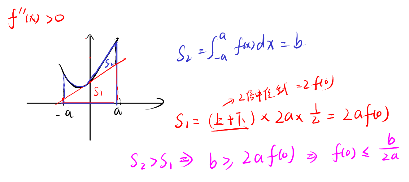
Original note figure 1
- Suppose $f$ is continuous on $[-a,a]$, twice differentiable in its interior, $a\gt0$, and $\int_{-a}^{a}f(x)\,dx=b$. Use the sign of the second derivative over the whole interval. For each nonzero interior $x$, Taylor’s formula with a Lagrange remainder gives $f(x)=f(0)+f'(0)x+\dfrac12 f''(\xi_x)x^2$, where $\xi_x$ lies between $0$ and $x$. If $f''\ge0$ throughout the interior, then $f(x)\ge f(0)+f'(0)x$. Extend this to the endpoints by continuity, integrate, and cancel the odd term to obtain $b\ge2af(0)$. If $f''\le0$, the result is $b\le2af(0)$. A pointwise expansion with an $o(x^2)$ remainder alone cannot control the integral over a fixed interval; the sign condition over the whole interval is essential.
When a higher derivative of moderate order is required but direct differentiation is difficult, the following methods are commonly available:
If finding $f^{(n)}(0)$, examine the function’s parity and check whether it is odd.
Differentiate and look for a pattern or regularity.
Use Taylor expansion directly, or differentiate once or twice and use it if a suitable form appears. For example:
$$ f(x)=ln(\sqrt{1+x^2}-x), \text{find } f^{(5)}(0) $$Direct differentiation or Taylor expansion is difficult, so differentiate once: $\to f'(x)=-\dfrac{1}{\sqrt{1+x^2}}$. Now the Taylor expansion of $(1+x)^{α}$ can be used, expanding directly through $-\dfrac{3}{8}x^4+o(x^4)$. Differentiation is then simple, giving $f^{(5)}=f'^{(4)}(0)=-9$.
Some common techniques for finding higher derivatives are listed below. They are usually used for series or integrals, so it is easy to overlook their use in differentiation; pay attention to this.
For ${F(x,\,y)=\dfrac{f(x)(\text{ or }f(y))}{ax^2-by^2}}$, use the difference of squares to arrange terms. For example:
$$ {F(x,\,y)=\dfrac{2x}{x^2-y^2}=\dfrac{1}{x+y}+\dfrac{1}{x-y}} $$Use $\dfrac{d^n}{dx^n}\left(\dfrac1x\right)=(-1)^n\dfrac{n!}{x^{n+1}}$ to handle $1/(x+y)$ and $1/(x-y)$ separately. For partial derivatives with respect to $x$, hold $y$ constant. For derivatives with respect to $y$, hold $x$ constant and account for the inner derivative $-1$ of $x-y$. Thus $\partial_x^nF=(-1)^nn![(x+y)^{-n-1}+(x-y)^{-n-1}]$, whereas $\partial_y^nF=(-1)^nn!(x+y)^{-n-1}+n!(x-y)^{-n-1}$.
Look flexibly for the form $1^{\infty}$ and check whether $\lim a(x)b(x)=A$, $lima(x)=0$, and $limb(x)=\infty$ hold. Then directly obtain
$$ lim(1+a(x))^{b(x)}=e^{A} $$. Note: after simplification, the $1$ here is the key, and many transformations are possible.
If the base is not $e$ but $a$, multiply by $lna$. For example:
$$ {\lim_{x\to+\infty}x^P(a^{\frac{1}{x}}-a^{\frac{1}{x+1}})} $$Factor out the common factor to obtain directly:
$$ {{\lim_{x\to+\infty}x^P\times a^{\frac{1}{x+1}}(a^{\frac{1}{x(x+1)}}-1)}\Rightarrow x^P\times a^{\frac{1}{x+1}}\times \dfrac{lna}{x(x+1)}} $$
- For limits of the form $\infty-\infty$, there are generally two methods: first, combine terms over a common denominator; second, when that is difficult, multiply numerator and denominator by the same expression to eliminate radicals and obtain the form $\dfrac{\infty}{\infty}$. There is also a less obvious method: factor or simplify, then cancel terms using a Taylor expansion. For example:
- Find $\lim_{x\to+\infty}[\sqrt[3]{1-x^6}+x^2]$. Factoring gives $\sqrt[3]{1-x^6}=-x^2(1-x^{-6})^{1/3}$. Using $(1-u)^{1/3}=1-u/3+O(u^2)$, we obtain $-x^2[1-1/(3x^6)+O(x^{-12})]+x^2=1/(3x^4)+O(x^{-10})\to0$.
- For an expression under a radical (or inside an absolute value), when taking the root (or introducing a square root of a square to remove an absolute value), always watch the sign of the value. In some problems involving limits with radicals, discontinuities, asymptotes, and similar topics, the answer is the maximum of an expression. In other words, always watch the sizes of particular expressions under the given conditions, since they can lead to different answers.
- For $\lim_{n\to\infty}\dfrac{1-x^{2n}}{1+x^{2n}}$, compare $|x|$ with $1$: the limit is $1$ for $|x|\lt1$, $0$ for $|x|=1$, and $-1$ for $|x|\gt1$.
- For $x^{2n+1}$, $x^{2n}$, and $x^n$, distinguish all real ranges and write a piecewise result when needed, as in $660_{19}$:
- If $-1\lt x\lt1$, all three sequences tend to $0$; if $x=1$, all are identically $1$.
- If $x=-1$, the first two sequences are identically $-1$ and $1$, while $x^n=(-1)^n$ oscillates and has no limit.
- If $x\gt1$, all three sequences tend to $+\infty$.
- If $x\lt-1$, then $x^{2n+1}\to-\infty$ and $x^{2n}\to+\infty$. The absolute value of $x^n$ tends to infinity, but its sign alternates, so it has neither a finite limit nor a signed infinite limit.
Parametric Curves, Extrema, and the Definition of a Differential
When differentiating parametric equations, always remember
$$ y=f(x),\,\,\, \begin{cases} x=\phi(t) \\y=\psi(t) \end{cases} $$- When $x$ and $y$ are differentiable functions of $t$ and $dx/dt\ne0$, we have $\dfrac{dy}{dx}=\dfrac{dy/dt}{dx/dt}$. If $y(t)$ is defined implicitly by $te^y+y+1=0$, first differentiate with respect to $t$: $e^y+(te^y+1)\dfrac{dy}{dt}=0$. Hence, when $te^y+1\ne0$, $\dfrac{dy}{dt}=-\dfrac{e^y}{te^y+1}$. Then divide by $dx/dt$.
- Discussing the continuity and differentiability of $f(x)$:
- For differentiability, transform it into $y=f(x)$ and solve, or examine $\frac{dy}{dx}$ to determine differentiability.
- For continuity, eliminate the parameter and examine $y=f(x)$ directly; differentiability of course guarantees continuity. Alternatively, check whether $\phi(t)$ and $\psi(t)$ are continuous, but this alone only guarantees a continuous parametric curve. If the parameter can also be written continuously as $t=t(x)$ in the range under discussion, then $f(x)=\psi(t(x))$ is continuous. For example, a continuous, locally strictly monotone $\phi$ has a continuous local inverse, so this method applies. Otherwise, first determine whether the curve defines a single-valued function.
- To find an oblique asymptote, identify the $x\to\infty$ limit and the corresponding $t$ values. Use $\dfrac{y(t)}{x(t)}$ to find $a$, then use $y(t)-ax(t)=b$. ($880_{base}-2.2.11$)
- To compare two radical expressions, raise both sides to the $x$th power.
- Compare $2^{\frac{1}{2}},\,\,\,3^{\frac{1}{3}}$. Simply cube both sides, or raise both to the sixth power, to obtain the result.
- If $f$ is differentiable on an interval, $f'(x)\ge0$, and equality holds at only finitely many points, then $f$ is strictly increasing. The equation $f'(x_0)=0$ only says that the first-order rate is zero; it does not prevent strict increase, as $f(x)=x^3$ illustrates. If $x_0$ is an interior local maximum and $f''(x_0)$ exists, then $f'(x_0)=0$ and $f''(x_0)\le0$. This does not require $f'$ to decrease monotonically throughout a neighborhood. The equation $f''(x_0)=0$ neither makes the function constant nor determines whether an extremum occurs: $x^4$, $-x^4$, and $x^3$ have, respectively, a local minimum, a local maximum, and no extremum at zero.
- For local and global extrema of $f$, examine nondifferentiable points as well as differentiable ones. The definition of an extremum requires neither differentiability nor continuity. For example, $f(0)=1$ and $f(x)=0$ elsewhere gives a discontinuous strict local maximum at zero. Under the usual graph-based definition, an inflection point requires continuity and a change of concavity across the point; it can also occur at a nondifferentiable point.
- At a nondifferentiable point, first compare function values using the definition of an extremum. If the function is continuous there and the derivative changes from positive on the left interval to negative on the right, the point is a strict local maximum; a change from negative to positive gives a strict local minimum. A nondifferentiable point is not stationary: a stationary point requires an existing first derivative equal to zero. For an inflection point, check for a change of concavity. When the graph of the second derivative is given, typically examine its signs on the neighboring intervals and also verify continuity at the point.
- At a differentiable point, $f'(x_0)=0$ already identifies a stationary point. If additionally $f''(x_0)\gt0$, it is a strict local minimum; if $f''(x_0)\lt0$, it is a strict local maximum. If $f''(x_0)=0$, the second-derivative test is inconclusive. For inflection points, $f''(x_0)=0$ only identifies a candidate. Under the appropriate third-order differentiability assumptions, the additional condition $f'''(x_0)\ne0$ ensures that the second derivative changes sign and establishes an inflection point.
- If a function is continuous on a finite closed interval, differentiable in its interior, and has exactly one interior local extremum, that point is the corresponding global extremum. In general, find a closed-interval maximum or minimum by comparing values at interior stationary points, nondifferentiable points, and the endpoints.
- For open or infinite intervals, also calculate endpoint limits or $\lim_{x\to\pm\infty}f(x)$. These limits may provide only a supremum or infimum, rather than an attained function value. Determine whether a maximum or minimum exists before comparing candidates.
- For a continuous function on a finite closed interval, if its only interior local extremum is a local maximum, the minimum must be attained at an endpoint; the analogous statement holds with maximum and minimum interchanged. This is useful in proofs and requires endpoints belonging to the domain.
- For a piecewise function, treat joining points separately instead of simply joining the derivative formulas from the interiors of the pieces. Differentiability first requires the function to be defined at the point. If the problem asks for an extension at an undefined point, assign its value first, then check continuity and the one-sided difference quotients. Even when differentiability of the whole function is given, determine the derivative at the join by definition and write the derivative in an appropriate piecewise form.
- For a polynomial, a root $a$ of $f(x)=0$ with multiplicity $m$ ($m\ge1$) loses one order of multiplicity upon differentiation. More generally, suppose there is a sufficiently smooth local factorization $f(x)=(x-a)^m h(x)$ with $h(a)\ne0$. Then $f'(x)=(x-a)^{m-1}[mh(x)+(x-a)h'(x)]$, and the bracket equals $mh(a)\ne0$ at $a$. Hence $a$ is a root of $f'$ of multiplicity $m-1$ when $m\ge2$; when $m=1$, $f'(a)\ne0$ and the point is no longer a root of the derivative.
- A condition of the form $f(x+C)-f(x)=AC+o(C)$ is a local expansion as the increment $C\to0$, with $x$ fixed. Set $C=\Delta x$, divide by $C$, and take the limit to obtain $A=f'(x)$. This is not a linear identity valid for increments of arbitrary size.
- For every fixed $x$, a function $f$ satisfies $f(x+y)-f(x)=(f(x)-1)y+o(y)$ as $y\to0$. Find $f(x)$.
- Divide by $y$ and take the limit to obtain $f'(x)=f(x)-1$, so the differential is $df=(f(x)-1)\,dx$. Rewrite the equation as $[e^{-x}(f(x)-1)]'=0$ and integrate to get $f(x)=1+Ce^x$. The term $o(y)$ belongs to the function increment, not to the differential itself.
- For every fixed $x$, a function $f$ satisfies $f(x+y)-f(x)=(f(x)-1)y+o(y)$ as $y\to0$. Find $f(x)$.
Mean Value Theorems
Constructing Auxiliary Functions from Derivative Rules
- Construct auxiliary functions for proofs. Common auxiliary functions are listed below.
Formula: $(uv)' = u'v + uv'$. Use it in reverse as follows:
- $[f^2(x)]'=2f(x)f'(x)$. Thus, when $f(x)f'(x)$ appears, set $F(x)=f^2(x)$, or use $F(x)=\tfrac12 f^2(x)$ to match the coefficient exactly.
- $[f(x) \cdot f'(x)]' = [f'(x)]^2 + f(x)f''(x)$. When you see $[f'(x)]^2 + f(x)f''(x)$, set $F(x) = f(x)f'(x)$.
- $[f(x)e^{\varphi(x)}]' = [f'(x) + f(x)\varphi'(x)]e^{\varphi(x)}$. When you see $f'(x) + f(x)\varphi'(x)$, set $F(x) = f(x)e^{\varphi(x)}$.
- $\varphi(x) = x \Rightarrow$ When you see $f'(x) + f(x)$, set $F(x) = f(x)e^x$.
- $\varphi(x) = -x \Rightarrow$ When you see $f'(x) - f(x)$, set $F(x) = f(x)e^{-x}$.
- $\varphi(x) = kx \Rightarrow$ When you see $f'(x) + kf(x)$, set $F(x) = f(x)e^{kx}$. Note: $(uv)'' = u''v + 2u'v' + uv''$ may also be tested.
- Formula: $\left(\frac{u}{v}\right)' = \frac{u'v - uv'}{v^2}$. Use it in reverse as follows:
- $\left[\frac{f(x)}{x}\right]' = \frac{f'(x)x - f(x)}{x^2}$ When you see $f'(x)x - f(x)$ ($x \neq 0$), set $F(x) = \frac{f(x)}{x}$.
- $\left[\frac{f'(x)}{f(x)}\right]' = \frac{f''(x)f(x) - [f'(x)]^2}{f^2(x)}$. When you see $f''(x)f(x) - [f'(x)]^2$ ($f(x) \neq 0$), set $F(x) = \frac{f'(x)}{f(x)}$.
- $(\ln f(x))' = \frac{f'(x)}{f(x)}, \quad \left(\frac{f'(x)}{f(x)}\right)' = \frac{f''(x)f(x) - [f'(x)]^2}{f^2(x)}$. When you see $f''(x)f(x) - [f'(x)]^2$ $(f(x) \gt 0)$, set $F(x) = \ln f(x)$.
Starting from Endpoints, Taylor Remainders, and Hidden Points
- If a proposition to be proved contains $a+b$ or $a-b$, try the $Lagrange$ mean value theorem. The appearance of $a+b$ calls for constructing an abstract function $f(x)$. If $Lagrange$ can be applied and $x\neq0$, Cauchy’s mean value theorem can then be used: $\dfrac{f'(\xi)}{2\xi}\times \dfrac{1}{f'(\eta)}\,=\,\dfrac{f(a)-f(b)}{a^2-b^2}\times\dfrac{a-b}{f(a)-f(b)}$
- For difficult proofs that Taylor expansion can simplify, such as proving $f(x) \leq \dfrac{1}{n!}g(x)$ or statements involving $f^{n(n\geq2)}$, consider the $Lagrange$ remainder formula.
Prove $\left|\dfrac{\sin x}{x}-1\right|\le\dfrac12|x|$. For $x\ne0$, use Taylor’s formula at zero with a Lagrange remainder:
$$ \sin x=\sin0+\cos0\,x-\frac{x^2\sin\xi}{2}=x-\frac{x^2\sin\xi}{2}, \qquad \min(0,x)\lt\xi\lt\max(0,x). $$Thus $\left|\dfrac{\sin x}{x}-1\right|=\left|-\dfrac{x\sin\xi}{2}\right|\le\dfrac12|x|$. For $x\gt0$, $\xi\in(0,x)$; for $x\lt0$, $\xi\in(x,0)$. Extending $\sin x/x$ continuously to the value $1$ at zero makes the inequality valid there as well.
- In proof problems involving mean value theorems, sometimes find hidden points: their existence alone can be enough to prove the result.
- A nonconstant function $f$ is continuous on $[a,b]$, differentiable on $(a,b)$, and satisfies $f(a)=f(b)=0$. Prove that its derivative is positive at some interior point and negative at another. Nonconstancy and the zero endpoint values guarantee a point $c\in(a,b)$ with $f(c)\ne0$. Apply Lagrange’s mean value theorem on $[a,c]$ and $[c,b]$ to obtain $f'(\xi_1)=\dfrac{f(c)}{c-a}$ and $f'(\xi_2)=-\dfrac{f(c)}{b-c}$, where $\xi_1\in(a,c)$ and $\xi_2\in(c,b)$. Both denominators are positive, so the derivatives have opposite signs: positive then negative if $f(c)\gt0$, and negative then positive if $f(c)\lt0$. This proves the claim.
Integration
Antiderivatives, Integrability, and Integral Mean Value Theorems
- For an antiderivative $F(x)$ and its derivative $f(x)$ in indefinite integration, we know the following:
- For the variable-limit integral $F(x)=\int_{a}^{x}f(t)\,dt$, existence implies continuity.
- Proof of the integral mean value theorem
Suppose $f$ is continuous on $[a,b]$, $a\lt b$, and its minimum and maximum are $m$ and $M$. The bounds $m(b-a)\le\int_a^b f(x)\,dx\le M(b-a)$ place the integral average in $[m,M]$. The intermediate value theorem then gives $\xi\in[a,b]$ such that $\int_a^b f(x)\,dx=f(\xi)(b-a)$.
To prove that there exists $\eta\in(a,b)$ such that $\int_{a}^{b}f(x)\,dx=f(\eta)(b-a)$, consider Lagrange’s mean value theorem. Because $f(x)$ is continuous, define $F(x)=\int_{a}^{x}f(t)\,dt$, giving $F(b)-F(a)=f(\eta)(b-a)\,\Rightarrow\,\int_{a}^{b}f(x)\,dx-0=f(\eta)(b-a),\,\,\eta\in(a,b)$.
The weighted form of the integral mean value theorem:
If $f(x),\,\,g(x)$ are continuous on $[a,b]$ and $g(x)$ does not change sign, then
$$ \int_{a}^{b}f(t)g(t)dt=f(\xi)\int_{a}^{b}g(t)dt,\,\,\xi\in[a,b] $$
During a proof, turn a constant into a variable, then use the integral mean value theorem and monotonicity to prove an inequality. For example:
- $f(x)$ is monotonically increasing. Prove ${\int_{a}^{b}xf(x)dx \geq \dfrac{a+b}{2}\int_{a}^{b}f(x)dx}$.
If $f$ is also continuous, turn the constant into a variable and define $F(x)=\int_a^x tf(t)\,dt-\dfrac{a+x}{2}\int_a^x f(t)\,dt$. For $a\lt x\lt b$, the integral mean value theorem supplies $\xi\in(a,x)$ such that
$$ F'(x)=\frac12\left[(x-a)f(x)-\int_a^x f(t)\,dt\right] =\frac{x-a}{2}[f(x)-f(\xi)]\ge0. $$Since $F(a)=0$, we obtain $F(b)\ge0$, which is the desired inequality. If only monotonicity is assumed, $f$ is still integrable on the finite closed interval, and we can use the direct identity
$$ 2(b-a)\left[\int_a^b xf(x)\,dx-\frac{a+b}{2}\int_a^b f(x)\,dx\right] =\int_a^b\int_a^b(x-t)[f(x)-f(t)]\,dt\,dx\ge0. $$Increasing monotonicity makes the integrand nonnegative, so the conclusion remains valid.
- $f(x)$ is monotonically increasing. Prove ${\int_{a}^{b}xf(x)dx \geq \dfrac{a+b}{2}\int_{a}^{b}f(x)dx}$.
- A continuous function $f(x)$ necessarily has an antiderivative $F(x)$. Proof: suppose $f$ is continuous on $[a,b]$ and define $F(x)=\int_a^x f(t)\,dt$. For $x,x+\Delta x\in(a,b)$ and $\Delta x\ne0$, the integral mean value theorem gives $\Delta F=\int_x^{x+\Delta x}f(t)\,dt=f(\xi)\Delta x$, where $\xi$ lies between $x$ and $x+\Delta x$. This holds for positive and negative increments. Divide by $\Delta x$ and let $\Delta x\to0$, so that $\xi\to x$. Continuity of $f$ gives $F'(x)=\lim_{\Delta x\to0}\Delta F/\Delta x=\lim_{\xi\to x}f(\xi)=f(x)$, proving that $F$ is an antiderivative of $f$.
- If $f(x)$ has a discontinuity of the first kind or an infinite discontinuity, it has no antiderivative $F(x)$.
- If $f(x)$ exists as a derivative, its antiderivative must be differentiable and continuous everywhere in its domain. When finding the antiderivative $F(x)$, pay attention to potential discontinuities (where $f(x)$ is piecewise), and use $\int f(x)+C$ to join the pieces of the antiderivative.
- When finding an indefinite integral, always include $+C$.
- Definite Riemann integrals on finite closed intervals
Integrability of $f(x)$ implies $|f(x)|\leq M$.
Remember additivity of definite integrals. For example, find ${\lim_{n\to\infty}\sum_{k=1}^{n}\int_{k}^{k + 1}f(x)}$. Pay attention to the information inside the summation; writing out several terms reveals ${\int_{k}^{k + 1}+\int_{k + 1}^{k + 2}+\dots=\lim_{n\to+\infty}\int_{1}^{n + 1}f(x)=\int_{1}^{+\infty}f(x)dx}$.
For the geometric meaning of a definite integral, any function value within each small subinterval can be used as its sampled value. For convenience we often choose the $i$th value, $f(\frac{i}{n})$, but we can also use the midpoint value $f(\frac{2i-1}{2n})$ or another value. The general formula is
$$ \int_{a}^{b} f(x) \,dx \,= \, \lim_{n \to \infty} \sum_{i=1}^{n}\,f(a+\frac{b-a}{n}i)\frac{b-a}{n} $$. Note that we can divide the interval into not only $n$ equal parts but also $2n, 3n\dots$; the definition remains unchanged. In particular, $\frac{b-a}{n}i$ must correspond to the width $\frac{b-a}{n}$.
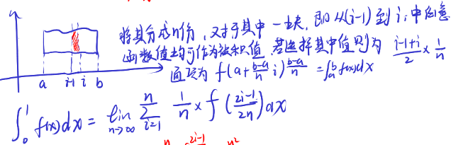
Original note figure 2 If $f$ is bounded on a finite closed interval $[a,b]$ and has only finitely many discontinuities, then $\int_a^b f(x)\,dx$ exists. Boundedness cannot be replaced merely by excluding infinite-limit discontinuities: unbounded oscillation also prevents proper Riemann integrability. For example, $\sin(1/x)/x$ with a value assigned at zero has only that one discontinuity and no infinite limit, yet it is unbounded near zero.
Sufficient conditions for the existence of a definite integral
- $f(x)$ is monotone on $I$.
- $f(x)$ is continuous on $I$.
- $f(x)$ is bounded on $I$ and has only finitely many discontinuities.
Necessary conditions for the existence of a definite integral
- $f(x)$ is bounded on $I$.
- The interval of integration has finite length.
For comparison problems, investigate the following possibilities (the list is incomplete, but it includes essentially everything that comes to mind):
Check whether oddness can simplify the expression, or whether splitting it simplifies some terms. For example,
$$ \int_{-\frac{1}{2}}^{\frac{1}{2}}\dfrac{x^2+x+1}{x^2+1} $$splits directly into a constant and an odd function, giving $1$.
Combine bounds, substitution, and parity when comparing integrals. For example, compare $M=\int_{-\pi/2}^{\pi/2}\sin^2x\cos x\,dx$ with $N=\int_{-\pi/2}^{\pi/2}(\sin^3x-\cos x)\,dx$. Set $u=\sin x$ in $M$ to get $M=\int_{-1}^1u^2\,du=2/3$. In $N$, $\sin^3x$ is odd, so $N=-\int_{-\pi/2}^{\pi/2}\cos x\,dx=-2$. Thus $M\gt N$. Before using a bound, verify that its pointwise inequality holds throughout the integration interval.
Discuss the function’s properties. A denominator whose behavior is already determined need not be discussed, simplifying the analysis. For example, for $\displaystyle\int_{0}^{1}\dfrac{(1+x)ln^2(1+x)}{x^2}\,dx$, directly examine the numerator.
Variable-Limit and Improper Integrals
- Variable-limit integrals
- The variable-limit integral $\int_{a}^{x}f(t)\,dt$ is a function of $x$.
- If $f(x)$ is integrable, then $F(x) = \int_{a}^{x}f(t)\,dt$ is continuous. Note that $F(x)$ need not be an antiderivative, and $f(x)$ need not be continuous: a function with finitely many discontinuities can also be integrable. Thus a variable-limit integral is necessarily continuous whenever it exists. The proof is as follows:
$f(x)$ is integrable, so $|f(x)|\leq M$. We have
$$ |F(x+\Delta x)-F(x)|=\left|\int_x^{x+\Delta x}f(t)\,dt\right|\le M|\Delta x| $$This estimate holds for both positive and negative $\Delta x$. Since $M|\Delta x|\to0$, the squeeze theorem gives $F(x+\Delta x)-F(x)\to0$, or $\lim_{\Delta x\to0}F(x+\Delta x)=F(x)$. Thus $F$ is continuous.
- If $f$ has a jump discontinuity at $x_0$, the left and right derivatives of $F$ there equal the corresponding one-sided limits of $f$. These limits differ, so $F$ is not differentiable at the point.
- If $f$ has a removable discontinuity at $x_0$, then $F$ is differentiable there and $F'(x_0)=\lim_{x\to x_0}f(x)$. This can differ from the assigned value $f(x_0)$, since changing an integrand at a single point does not change its integral.
- For differentiation of a variable-limit integral of an abstract function, such as $\int_{F_2(x)}^{F_1(x)}f(g(x)-h(t))dt$, first substitute for the inner expression $g(x)-h(t)$ to make differentiation easier. See $(888_{comp}(3.3.8))$.
- Differentiate $H(x)=\int_0^{x^2}tf(x^2-t^2)\,dt$. One method is to find an antiderivative with respect to $t$ and evaluate it at the endpoints. Alternatively, set $u=x^2-t^2$, so $du=-2t\,dt$. The endpoint $t=0$ gives $u=x^2$, and $t=x^2$ gives $u=x^2-x^4$. Hence $H(x)=\dfrac12\int_{x^2-x^4}^{x^2}f(u)\,du$. If $f$ is continuous, the variable-limit differentiation rule gives $H'(x)=xf(x^2)-(x-2x^3)f(x^2-x^4)$.
- If ${f(x)}$ is odd, then $\int_{a}^{x}f(t)dt$ is necessarily even. If $f(x)$ is even, but $a\neq0$ or $F(a)\neq0$, we cannot conclude that $\int_{a}^{x}f(t)dt$ is odd.
- For convergence or divergence of improper integrals over infinite intervals, such as $\int_{-\infty}^{\infty}e^{|x|}sinx$, remember that the usual odd-function property does not apply here. If the function’s integral diverges at one end, adding or subtracting two divergent integrals still leaves divergence.
- For limits of variable-limit integrals, matching convergence or divergence behavior alone does not justify equivalent substitution. If $f(t)\sim g(t)$ as $t\to0^+$, both functions are integrable near zero, and $g$ keeps one sign on that side with a nonzero denominator integral, then $\int_0^x f(t)\,dt\sim\int_0^x g(t)\,dt$ as $x\to0^+$. Check the corresponding conditions separately for the other side. A Taylor expansion also requires control of the remainder over the interval of integration. For example, if $f(t)=\sum_{k=0}^m a_kt^k+o(t^m)$ with nonnegative integer $m$, then $\int_0^x f(t)\,dt=\sum_{k=0}^m\dfrac{a_k}{k+1}x^{k+1}+o(x^{m+1})$. This preserves the correct leading coefficient as well as the convergence behavior.
Radical Signs, Integration by Parts, and Interval Symmetry
- Calculating integrals
- Always watch the sign when taking square roots. Because of restrictions on the integrand’s domain, if $x$ must be moved inside a radical or taken out of it and $x$ is negative, add a minus sign.
- A curve passes through $(-2, 0)$ and has slope ${\dfrac{1}{x\sqrt{x^2-1}}}$ at every point. Find the curve.
Nonnegativity inside the radical gives two possible ranges for $x$. Use the point on the curve to determine the specific range of $x$, then find the indefinite integral. Set $x=sect$, giving
$$ {\dfrac{1}{x\sqrt{x^2-1}}dx \Rightarrow \int\dfrac{sect\,tant}{sec\,(-tant)}dt=-arccos(\frac{1}{x})+C} $$. Pay particular attention to $-tant$ here. The range of $x$ obtained above gives $tant\lt 0$, so we need $\sqrt{tan^2t}=-tant$. This applies not only to trigonometric functions but also to $x$.
- Evaluate ${\displaystyle\int_{-\tfrac{\pi}{2}}^{\tfrac{\pi}{2}}\int_{0}^{Rcos\theta}\dfrac{r}{\sqrt{R^2-r^2}}\,dr}$.
- Finding an antiderivative of the integrand is straightforward, giving ${R-Rsin\theta}$. However, the outer ${\theta}$ range contains negative values, so this becomes ${R-R|sin\theta|}$. Then integrate.
- A curve passes through $(-2, 0)$ and has slope ${\dfrac{1}{x\sqrt{x^2-1}}}$ at every point. Find the curve.
- To split terms and cancel them through integration by parts, first look for a part whose derivative matches another part. Typical forms include $e^{f(x)}$ multiplied by $\sin x$, $\cos x$, or $\tan x$. For example, $(1+\tan x)^2=\sec^2x+2\tan x$ suggests using $(\tan x)'=\sec^2x$ to pair terms, but retain the coefficient $2$ and match the other factors before claiming cancellation. $(\mathrm{Zhang}_{base}(9.5,\,T_{9.11}),\,880_{base}(3.3.4.6),\,880_{comp}(3.3.3))$
- If an abstract integral such as $\int x^{n-1}\sqrt{1+x^n}dx$ appears, seeing $n-1$ and $n$ should suggest matching a differential.
- After substitution, integrate $f(t)dg(t)$ by parts to turn it into $g(t)df(t)$. Example: ($\mathrm{Zhang}_{base}9.7$).
- Interval reflection: for $f(x)g(sinx),\,\,f(x)g(cosx)$, and sometimes expressions containing ${f(x)e^x}$, if integration is difficult, tentatively check whether reflection of the interval can be used. Examples: ($\mathrm{Zhang}_{base}9.18,\,\,9.12$, ${\mathrm{Wu}_{comp}P_{115}-9}$).
- For $\dfrac{1}{1+sinx},\,\,\dfrac{1}{1+cosx}$ and similar expressions, frequently use rationalization of the numerator and denominator, multiplying both by the same expression.
- Example: $\int\dfrac{x}{1+sinx}$. Rationalize the denominator directly; when $xf(sinx/tanx/cosx)$ appears, use interval reflection.
- Always watch the sign when taking square roots. Because of restrictions on the integrand’s domain, if $x$ must be moved inside a radical or taken out of it and $x$ is negative, add a minus sign.
Inverse Trigonometric Branches and Trigonometric Integrals
- When substituting in an integral, check whether the inverse function’s interval must be split. For expressions such as $arcsinsinx,\,\,arctantanx$, watch the range; check whether the function is monotone.
Evaluate
$$ {\int_{0}^{1}x\,arcsin(2\sqrt{x-x^2})\,dx} $$.
For an expression such as ${\sqrt{x-x^2}}$, set ${x=sin^2\theta}$, giving
$$ {\int_{0}^{\frac{\pi}{2}}sin^2\theta\cdot arcsin(sin2\theta)\cdot2sin\theta\cdot cos\theta\,d\theta} $$. Because $\arcsin(\sin 2\theta) =\begin{cases}2\theta, & 0 \leq \theta \leq \frac{\pi}{4} \\\pi - 2\theta, & \frac{\pi}{4} \leq \theta \leq \frac{\pi}{2}\end{cases}$, we have
$$ {I = \int_0^{\frac{\pi}{4}} 2 \sin^3 \theta \cos \theta (2\theta) \, d\theta + \int_{\frac{\pi}{4}}^{\frac{\pi}{2}} 2 \sin^3 \theta \cos \theta (\pi - 2\theta) \, d\theta} $$. At this point, $I_1=\int_0^{\pi/4}\theta\,d(\sin^4\theta)$ and $I_2=\int_{\pi/4}^{\pi/2}(\pi/2-\theta)\,d(\sin^4\theta)$. Integration by parts gives $I_1=\pi/16-\int_0^{\pi/4}\sin^4\theta\,d\theta$ and $I_2=-\pi/16+\int_{\pi/4}^{\pi/2}\sin^4\theta\,d\theta$. In the latter integral set $u=\pi/2-\theta$. Then $I=\int_0^{\pi/4}(\cos^4u-\sin^4u)\,du=\int_0^{\pi/4}\cos2u\,du=1/2$.
Some commonly used inverse-trigonometric formulas are listed here:
- ${\begin{align} \arctan x+\arctan y&=\arctan\frac{x+y}{1-xy}\quad(xy\lt 1)\\ &=\pi+\arctan\frac{x+y}{1-xy}\quad(x\gt 0,xy\gt 1)\\ &=-\pi+\arctan\frac{x+y}{1-xy}\quad(x\lt 0,xy\gt 1)\\ \end{align}}$
- ${\begin{align} \arctan x-\arctan y&=\arctan\frac{x-y}{1+xy}\quad(xy\gt -1)\\ &=\pi+\arctan\frac{x-y}{1+xy}\quad(x\gt 0,xy\lt -1)\\ &=-\pi+\arctan\frac{x-y}{1+xy}\quad(x\lt 0,xy\lt -1)\\ \end{align}}$
- When ${xy = 1}$ and ${x \ne 0}$, ${\arctan x + \arctan \dfrac{1}{x} = \begin{cases} \dfrac{\pi}{2}, & x \gt 0 \\\\-\dfrac{\pi}{2}, & x \lt 0\end{cases}}$.
- When ${xy = -1}$ and ${x \ne 0}$, we have ${{\arctan x - \arctan \left( -\dfrac{1}{x} \right) = \arctan x + \arctan \dfrac{1}{x} = \begin{cases} \dfrac{\pi}{2}, & x \gt 0 \\\\ -\dfrac{\pi}{2}, & x \lt 0 \end{cases}}}$.
- Use the integration properties of odd and even functions, splitting the expression if necessary.
- For $\dfrac{1}{a^2+x^2}dx$, recognize its general structure, as in $\dfrac{1}{x^2-x+1}\rightarrow \dfrac{1}{(x-\frac{1}{2})^2+(\frac{\sqrt{3}}{2})^2}$. Be sure to match the differential $d(x-\frac{1}{2})$ here; similarly, for $dAx$, supply the constant factor.
- For expressions such as $R(-sinx,\,cosx)=-R(sinx,\,cosx)\dots$, learn substitution and matching differentials. Also remember the universal substitution formulas $(P_{289})$. See ($\mathrm{Wu}_{base}P_{81}-13,14$).
- For a trigonometric rational function satisfying $R(-\sin x,-\cos x)=R(\sin x,\cos x)$, use $u=\tan x$ on suitable intervals to obtain a rational integral. Without this symmetry, the universal substitution $u=\tan(x/2)$ remains available. Account for the relevant branches and any zeros of the denominators. $(1k_{base}14.20)$
- For ${sinax \times cosbx}$, consider product-to-sum identities; sum-to-product identities can likewise be used in reverse.
- $\sin x\cos(nx)=\tfrac12[\sin((1+n)x)+\sin((1-n)x)]$, so $\int\sin x\cos(nx)\,dx=\tfrac12\int[\sin((1+n)x)+\sin((1-n)x)]\,dx$.
- For $e^{ax}cos/sinbx$, apply the formula directly $(\mathrm{Zhang}_{base}{285})$. See ($\mathrm{Zhang}_{base}(10.4)$).
- For $\int\dfrac{a\sin x+b\cos x}{c\sin x+d\cos x}\,dx$, where $c,d$ are not both zero, rearrange terms to match a differential. Solve $Ac-Bd=a$ and $Ad+Bc=b$ for $A,B$, then write the integrand as $\dfrac{A(c\sin x+d\cos x)+B(c\cos x-d\sin x)}{c\sin x+d\cos x}$. On an interval where the denominator is nonzero, use $d\ln|c\sin x+d\cos x|$ to obtain the antiderivative $Ax+B\ln|c\sin x+d\cos x|+C$. Examples: Li/Fan (3.40), $880_{base}(3.3.3,\,3.3.4)$.
Reduction of Order, Area, and Special Functions
For some variable-limit integrals such as $f(x)\int_{a}^{x}g(t)dt$, or higher derivatives $f^{n}$, try integration by parts to reduce the order and find a solution ($\mathrm{Zhang}_{base}11.6,\,1k_{base}{10.7}$).
Become familiar with common trigonometric identities and their coefficients, for example $(1+\tan x)^2=1+2\tan x+\tan^2x=\sec^2x+2\tan x$.
If the problem asks for the area associated with a function, remember that area is nonnegative: watch the function’s sign on the specified interval and, when necessary, calculate by taking a limit in the definition of the definite integral.
A good example is $y=e^{-x}sinx$. Calculate the area on one interval and then use the definition of the definite integral, namely
$$ \lim_{n\to \infty}\sum_{k=0}^{n}\int_{k\pi}^{(k+1)\pi}e^{-x}|sinx|dx $$. Do not take this for granted: always watch the function’s sign, and keep paying attention to its sign.
Pay attention to the integral ${\int_{a}^{b}dx\int_{x}^{b}f(x)f(y)dy}$. Set $F(x)=\int_{x}^{b}f(x)dx$, then match differentials:
$$ {\int_{a}^{b}dx\int_{x}^{b}f(x)f(y)dy=\int_{a}^{b}[\int_{x}^{b}f(y)dy]\,d\,[-\int_{x}^{b}f(y)dy]} $$.
The Beta and Gamma functions:
- For expressions of the form ${\displaystyle \int_{0}^{+\infty}x^{\alpha-1}e^{-x}dx,\,2\int_{0}^{+\infty}t^{2\alpha-1}e^{-t^2}dt}$, consider the ${\Gamma}$ function. Some resulting identities are ${\Gamma(\alpha+1)=\alpha\Gamma(\alpha),\,\Gamma(n+1)=n!,\,\Gamma(\dfrac{1}{2})=\sqrt{\pi}}$.
- For $p\gt0$ and $q\gt0$, the Beta function has two common integral forms: $B(p,q)=\int_0^\infty\dfrac{t^{p-1}}{(1+t)^{p+q}}\,dt=\int_0^1u^{p-1}(1-u)^{q-1}\,du$. Its relation to the Gamma function is $B(p,q)=\dfrac{\Gamma(p)\Gamma(q)}{\Gamma(p+q)}$. These forms often appear after trigonometric substitution.
Generalization: ${\displaystyle \int_0^{+\infty} \frac{x^{p-1}}{1 + x^q} \, \mathrm{d}x = \frac{\pi}{q\,\sin\left( \frac{p\pi}{q} \right)}, \quad 0 \lt p \lt q}$.
Evaluate
$$ {\int_{0}^{\frac{\pi}{2}}\dfrac{sin^2x\,cos^2x}{(sinx+cosx)^6} dx} $$. The integrand satisfies $R(-\sin x,-\cos x)=R(\sin x,\cos x)$. Set $t=\tan x$ and use $dx=dt/(1+t^2)$ to obtain:
$$ {\int_0^{\infty} \dfrac{t^2}{(1+t)^6}dt=B(3,3) = \dfrac{\Gamma(3)\Gamma(3)}{\Gamma(6)} = \dfrac{2! \cdot 2!}{5!} = \dfrac{4}{120} = \dfrac{1}{30}} $$
Reciprocal Substitutions and Parameter Integrals
- Consider $\int_0^\infty\dfrac{x^2}{1+x^4}\,dx$. Set $x=1/t$, so $dx=-dt/t^2$. The integrand together with its differential becomes $-dt/(1+t^4)$, while the endpoints change from $0,\infty$ to $\infty,0$. Thus $\int_0^\infty\dfrac{x^2}{1+x^4}\,dx=\int_0^\infty\dfrac1{1+t^4}\,dt$. Adding the two forms and dividing by two reduces the desired integral to $\dfrac12\int_0^\infty\dfrac{1+x^2}{1+x^4}\,dx$. For $\int_0^\infty\dfrac{1+x^2}{1+x^4+ax^2}\,dx$ with $a\gt-2$, divide numerator and denominator by $x^2$, then look for $d(x+1/x)$ or $d(x-1/x)$. Here the numerator matches $d(x-1/x)=(1+x^{-2})\,dx$.
Evaluate ${\displaystyle \int_{0}^{+\infty}\dfrac{1}{1+x^6}}$ (${\mathrm{Wu}_{comp}P_{102}-\text{note}}$). *
$$ \begin{aligned}\int \frac{1}{1+(x^2)^3}\,dx&= \int \frac{1}{(1+x^2)(1 - x^2 + x^4)}\,dx\\&= \int \frac{(1+x^2)-x^2}{(1+x^2)(1 - x^2 + x^4)}\,dx\\&= \int\Bigl(\frac{1}{1 - x^2 + x^4} - \frac{x^2}{1 + x^6}\Bigr)\,dx\\&= \int \frac{1}{1 - x^2 + x^4}\,dx \;-\; \int \frac{x^2}{1 + x^6}\,dx\\&= \tfrac12\int \frac{1 + x^2 - x^2 + 1}{1 - x^2 + x^4}\,dx \;-\; \tfrac13\int \frac{1}{1+(x^3)^2}\,d(x^3)\\&= \tfrac12\int \frac{1 + x^2}{1 - x^2 + x^4}\,dx \;+\; \tfrac12\int \frac{1 - x^2}{1 - x^2 + x^4}\,dx \;-\; \tfrac13\int \frac{1}{1+(x^3)^2}\,d(x^3)\\&= \tfrac12\int \frac{\tfrac1{x^2}+1}{\tfrac1{x^2}-1+x^2}\,dx \;+\; \tfrac12\int \frac{\tfrac1{x^2}-1}{\tfrac1{x^2}-1+x^2}\,dx \;-\; \tfrac13\arctan(x^3)\\&= -\tfrac12\int \frac{1}{\bigl(\tfrac1x-x\bigr)^2+1}\,d\Bigl(\tfrac1x - x\Bigr)\;-\;\tfrac12\int \frac{1}{\bigl(\tfrac1x+x\bigr)^2-3}\,d\Bigl(\tfrac1x + x\Bigr)\;-\;\tfrac13\arctan(x^3)\\&= -\tfrac12\arctan\!\Bigl(\tfrac1x - x\Bigr)\;-\;\tfrac1{4\sqrt3}\ln\!\Bigl|\frac{\tfrac1x + x - \sqrt3}{\tfrac1x + x + \sqrt3}\Bigr|\;-\;\tfrac13\arctan(x^3)+C\\\end{aligned} $$With $u=1/x-x$ and $v=1/x+x$, we have $x^{-2}-1+x^2=u^2+1=v^2-3$. Let $F(x)$ denote the antiderivative above. Taking endpoint limits for $x\gt0$ gives $F(0^+)=-\pi/4$ and $F(+\infty)=\pi/12$, hence $\int_0^\infty\dfrac1{1+x^6}\,dx=\pi/3$.
Of course, these integrals can also be evaluated using the generalized ${Beta}$-function formula.
- Evaluate $\int_0^1\dfrac{x^t}{\ln x}\,dx$. As $x\to1^-$, $x^t/\ln x\sim1/(x-1)$, so for every real $t$ this improper integral diverges at the right endpoint and has no finite value.
- Feynman’s parameter-differentiation method applies to a convergent family. For example, for $t\gt-1$, define $J(t)=\int_0^1\dfrac{x^t-1}{\ln x}\,dx$. Cancellation in the numerator makes the singularity at $x=1$ removable. On any compact parameter interval $[a,b]\subset(-1,\infty)$, the parameter derivative $x^t$ is dominated by the integrable function $x^a$, so differentiation under the integral sign is justified. Thus $J'(t)=\int_0^1x^t\,dx=\left.\dfrac{x^{t+1}}{t+1}\right|_0^1=\dfrac1{t+1}$. Integrating and using $J(0)=0$ gives $J(t)=\ln(1+t)$.
- Evaluate $\int_0^1\dfrac{x^7-x^3}{\ln x}\,dx$.
- Write the numerator as $(x^7-1)-(x^3-1)$ and use the convergent family above to obtain $J(7)-J(3)=\ln8-\ln4=\ln2$.
Using Green’s Theorem in Reverse on Disks
- Sometimes an integral is difficult and involves a disk together with properties of first and second derivatives. Consider using Green’s theorem or the divergence theorem in reverse: turn an area integral into a line integral, then simplify using the problem’s conditions to calculate the result.
- The function $f(x,y)$ has continuous second partial derivatives on the disk $D=\{(x,y):x^2+y^2\le1\}$ and satisfies $(f_{xx}+f_{yy})e^{x^2+y^2}=1$. Find $I=\iint_D(xf_x+yf_y)\,dx\,dy$.
Let $D_r=\{(x,y):x^2+y^2\le r^2\}$ and let $L_r$ be its counterclockwise boundary. The full disk uses the angular range $0\le\theta\le2\pi$, so
$$ I=\int_0^1 r\,dr\int_0^{2\pi} [r\cos\theta\,f_x(r\cos\theta,r\sin\theta)+r\sin\theta\,f_y(r\cos\theta,r\sin\theta)]\,d\theta. $$On $L_r$, $dx=-r\sin\theta\,d\theta$ and $dy=r\cos\theta\,d\theta$. Thus the inner integral is $\oint_{L_r}(-f_y\,dx+f_x\,dy)$. Green’s theorem and the given condition yield
$$ \begin{aligned} I&=\int_0^1 r\,dr\iint_{D_r}(f_{xx}+f_{yy})\,dA\\ &=\int_0^1 r\,dr\int_0^{2\pi}\int_0^r e^{-\rho^2}\rho\,d\rho\,d\theta\\ &=\pi\int_0^1 r(1-e^{-r^2})\,dr =\frac{\pi}{2e}. \end{aligned} $$
- The function $f(x,y)$ has continuous second partial derivatives on the disk $D=\{(x,y):x^2+y^2\le1\}$ and satisfies $(f_{xx}+f_{yy})e^{x^2+y^2}=1$. Find $I=\iint_D(xf_x+yf_y)\,dx\,dy$.
Multivariable Differentiation
Continuity, Partial Derivatives, and Differentiability
Continuity of a multivariable function at a point is equivalent to the limit existing and equaling the function value, provided that the function is defined at that point. Existence of the limit alone is insufficient. Continuity does not imply existence of partial derivatives or differentiability.
Partial derivatives describe rates of change along their respective coordinate axes. Different partial derivatives need not be equal, and directional derivatives in different directions need not agree. Existence of partial derivatives does not imply differentiability; differentiability implies both partial derivatives and continuity. The gradient is the vector of partial derivatives; its existence alone does not establish a total differential. A sufficient condition for differentiability at a point is that all partial derivatives exist nearby and are continuous at that point. Differentiability guarantees one linear approximation valid for every approach to the point, but does not require continuous partial derivatives.
First consider a function with partial derivatives but without differentiability:
$$ f(x,y)= \begin{cases} \dfrac{x^2y}{x^4+y^2},&(x,y)\ne(0,0),\\ 0,&(x,y)=(0,0). \end{cases} $$It vanishes along both coordinate axes, so $f_x(0,0)=f_y(0,0)=0$. Along $y=x^2$ with $x\ne0$, however, $f(x,x^2)=1/2$. Thus it has no limit at the origin and is neither continuous nor differentiable there.
To see that differentiability does not imply continuous partial derivatives, consider
$$ g(x,y)= \begin{cases} x^2\sin(1/x),&x\ne0,\\ 0,&x=0. \end{cases} $$Let $\rho=\sqrt{x^2+y^2}$. Since $|g(x,y)|/\rho\le x^2/\rho\le\rho\to0$, the function is differentiable at the origin with zero total differential. On the other hand, for $x\ne0$,
$$ g_x(x,y)=2x\sin(1/x)-\cos(1/x), $$which has no limit at the origin. Hence this partial derivative is discontinuous.
If only $f_x(x_0,y_0)$ and $f_y(x_0,y_0)$ are known to exist, distinguish information along the axes from information throughout a disk. By definition,
$$ f_x(x_0,y_0)=\lim_{x\to x_0} \frac{f(x,y_0)-f(x_0,y_0)}{x-x_0}. $$With $y=y_0$ fixed, this is a single-variable derivative, whose existence gives continuity along that coordinate direction:
$$ \lim_{x\to x_0}f(x,y_0)=f(x_0,y_0). $$The same applies with $x=x_0$ fixed. Being defined and continuous on those axis intervals does not establish a domain containing a two-dimensional disk, a two-dimensional limit, or continuity at the point. A neighborhood domain is usually a separate assumption in the problem, not a consequence of partial derivatives existing.
Implicit Functions and Mixed Partial Derivatives
For $F(x,y)=0$, suppose $F$ has continuous first partial derivatives near $(x_0,y_0)$, $F(x_0,y_0)=0$, and $F_y(x_0,y_0)\ne0$. The implicit function theorem gives a unique local differentiable function $y=y(x)$ satisfying
$$ y'(x)=-\frac{F_x(x,y(x))}{F_y(x,y(x))}. $$When $F_y=0$, an implicit function may still exist, so examine the equation itself. An indeterminate derivative quotient, or the existence of a limit of such a quotient, does not by itself prove that an implicit function exists.
When using the definition of a partial derivative, fix the other variable. For second- or higher-order mixed partials, initially retain that other variable as a parameter. For example,
$$ f_x(x_0,y)=\lim_{h\to0} \frac{f(x_0+h,y)-f(x_0,y)}{h}, \qquad f_{xy}(x_0,y_0)= \left.\frac{d}{dy}f_x(x_0,y)\right|_{y=y_0}. $$The increment $h$ tends to zero. Do not substitute every coordinate of the fixed point before completing the required differentiations.
The Total Differential and Linear Approximation
Let the base point be $(x_0,y_0)$ and set $\rho=\sqrt{(\Delta x)^2+(\Delta y)^2}$. Differentiability at this point means that constants $A,B$ exist such that
$$ \begin{aligned} \Delta z&=f(x_0+\Delta x,y_0+\Delta y)-f(x_0,y_0),\\ \Delta z&=A\Delta x+B\Delta y+o(\rho), \qquad \rho\to0. \end{aligned} $$Equivalently,
$$ \lim_{(\Delta x,\Delta y)\to(0,0)} \frac{\Delta z-A\Delta x-B\Delta y}{\rho}=0. $$Then $A=f_x(x_0,y_0)$ and $B=f_y(x_0,y_0)$, and the total differential is $dz=A\,dx+B\,dy$. The distance in the remainder must be measured from the base point.
For example, when a problem uses a higher-order infinitesimal as a denominator, explicitly name it $q(x,y)$: it is nonzero in a punctured neighborhood and satisfies $q=o(r)$, where $r=\sqrt{(x-a)^2+(y-b)^2}$. Little-o notation describes a class of remainders, not one specified function. Suppose
$ \lim_{(x,y)\to(a,b)} \frac{f(x,y)-f(a,b)+3(x-a)-4(y-b)}{q(x,y)} =C,\qquad 0\lt |C|\lt\infty. $
Denoting the numerator by $N(x,y)$ gives
$$ \frac{N(x,y)}r =\frac{N(x,y)}{q(x,y)}\,\frac{q(x,y)}r \longrightarrow C\cdot0=0. $$Thus $N=o(r)$, or
$$ f(x,y)-f(a,b)=-3(x-a)+4(y-b)+o(r). $$The definition now establishes differentiability at $(a,b)$, with $f_x(a,b)=-3$ and $f_y(a,b)=4$. This is a different quotient with a different limit; the given constant $C$ itself has not changed to zero.
Finding Local and Global Extrema
When finding local extrema and global maximum or minimum values, collect candidate points before classifying them:
- Inspect interior points where differentiability or partial derivatives fail, and solve for stationary points, where all first partial derivatives exist and vanish. Denote the interior candidates by $M_i$. Failure of differentiability does not make a point stationary, and a stationary point still requires classification.
- If constraints are present, discard candidates in $M_i$ that violate them. Use Lagrange multipliers on smooth constraints or boundaries where the regularity conditions hold, obtaining candidates $M_j$.
- Inspect every endpoint, corner, and singular point where a constraint fails its regularity condition, denoting these candidates by $M_k$. Checking a few arbitrary endpoints is insufficient.
- Provided the global extrema are attained and the candidates are complete, compare the function values at $M_i,M_j,M_k$. These symbols designate candidates, not points already proved to be local extrema.
A global extremum is a local extremum relative to the feasible domain. A boundary extremum may be only a constrained local extremum, not an unconstrained extremum in an open neighborhood. Even a unique interior local extremum need not be a global extremum. The boundary and actual attainment still need attention.
Given $f(x,y)$ on a region $D$, first separate the interior and boundary. If $D$ has an interior, find the interior candidates, then substitute the boundary conditions to obtain a single-variable function $g(x)$, find its candidate values, and compare. Use Lagrange multipliers when the boundary function is difficult; if $D$ is itself an equality constraint, work directly on it. For $D=\{x\ge0,y\ge0\}$, the boundary consists of the two half-axes $x=0,y\ge0$ and $y=0,x\ge0$, with these ranges retained.
Lagrange Multipliers and Representative Examples
When Lagrange equations resist direct elimination, try arranging them as a homogeneous linear system in the original variables:
$$ \begin{cases} \phi_1(\lambda)x+\mu_1(\lambda)y=0,\\ \phi_2(\lambda)x+\mu_2(\lambda)y=0. \end{cases} $$First check whether $(0,0)$ satisfies the constraint. If the constraint excludes it and the candidate must satisfy this system, require a nonzero solution and set the coefficient determinant to zero. Find $\lambda$ first, then $(x,y)$. The mere presence of a constraint does not exclude the zero solution. Multiplying or dividing derivative equations, or multiplying them by the corresponding variables and adding, may also simplify the calculation. Check zero denominators separately before dividing.
Example: a planar section of an ellipsoid. Find the semimajor and semiminor axes of the ellipse cut from $f(x,y,z)=x^2/3+y^2/2+z^2=1$ by $D(x,y,z)=x+y+z=0$.
The cutting plane passes through the ellipsoid’s center, so the ellipse is centered at the origin. The origin lies inside its enclosed region, not on the ellipse itself. The semiaxes are the largest and smallest distances from the center, so optimize $d^2=x^2+y^2+z^2$. With both constraints, use
$$ L=x^2+y^2+z^2 +\lambda\left(\frac{x^2}{3}+\frac{y^2}{2}+z^2-1\right) +\mu(x+y+z). $$The equations $L_x=L_y=L_z=0$ are
$$ \begin{cases} (2+2\lambda/3)x+\mu=0,\\ (2+\lambda)y+\mu=0,\\ (2+2\lambda)z+\mu=0. \end{cases} $$Eliminate $\mu$ using $L_x-L_y=0$ and $L_y-L_z=0$, then substitute $z=-x-y$:
$$ \begin{cases} (2+2\lambda)x+(4+3\lambda)y=0,\\ (6+2\lambda)x+(-6-3\lambda)y=0. \end{cases} $$Here $(x,y)=(0,0)$ would force $z=0$, violating the ellipsoid constraint. Thus the system requires a nonzero solution:
$$ \begin{vmatrix} 2+2\lambda&4+3\lambda\\ 6+2\lambda&-6-3\lambda \end{vmatrix}=0 \quad\Longrightarrow\quad 3\lambda^2+11\lambda+9=0, \qquad \lambda=\frac{-11\pm\sqrt{13}}6. $$Only the lengths are required, so there is no need to recover each coordinate. Multiply the three stationary equations by $x,y,z$, respectively, and add. The constraints give $2d^2+2\lambda=0$, hence $d^2=-\lambda$. The ellipse is compact and distance is continuous, so the semimajor and semiminor axes are, respectively,
$$ \sqrt{\frac{11+\sqrt{13}}6}, \qquad \sqrt{\frac{11-\sqrt{13}}6}. $$Example: an arc maximizing a line integral. Choose an arc $L$ on the counterclockwise-oriented ellipse $C:x^2/4+y^2=1$ to maximize $\int_L(dx+2\,dy)$.
Since
$$ \int_L(dx+2\,dy)=(x+2y)\big|_A^B, $$choose the starting point $A$ to minimize $x+2y$ and the endpoint $B$ to maximize it. Lagrange multipliers for the ellipse give the minimum $-2\sqrt2$ and maximum $2\sqrt2$, attained at $A=(-\sqrt2,-1/\sqrt2)$ and $B=(\sqrt2,1/\sqrt2)$. The counterclockwise arc from $A$ to $B$ gives the maximum integral $4\sqrt2$.
A standard guarantee of global extrema is that $D$ is nonempty, closed, and bounded, and the function is continuous on $D$. Existence of second partial derivatives alone is insufficient. Even a smooth function on an open or unbounded region may fail to attain a maximum or minimum.
Provided the global extrema are attained, if $F(x,y)$ has no interior local extrema—all candidates satisfying $F_x=F_y=0$ have been ruled out and points with missing partial derivatives also fail the extremum definition—the global extrema must occur on the boundary. This parallels checking interior candidates and endpoints on a closed interval. Without an existence guarantee, there may be only a supremum or infimum, or the function may be unbounded; boundary extrema need not exist.
When the Hessian Test Is Inconclusive
At a stationary point with continuous second partial derivatives, write $A=f_{xx}$, $B=f_{xy}$, and $C=f_{yy}$. If $AC-B^2=0$, the second-derivative test is inconclusive; try a higher-order Taylor expansion or path analysis.
For a single-variable restriction with a first nonzero derivative and all preceding derivatives zero at the candidate, an odd first nonzero order rules out an extremum. An even order gives a minimum or maximum according to its sign. The relevant Taylor hypotheses are needed: the existence of some nonzero even-order derivative is not a necessary condition for every possible extremum. For multivariable functions, paths can rule out extrema, but even checking every straight-line path is generally insufficient to prove one.
Example: For $f(x,y)=x^2+y^2-6x+10$, examine $(2,0)$ and the function’s extrema. Completing the square gives
$$ f(x,y)=(x-3)^2+y^2+1, \qquad f_x=2x-6,\quad f_y=2y. $$At $(2,0)$, $f_x=-2$, so this point is neither stationary nor a local extremum. The unique stationary point is $(3,0)$, where the strict global minimum is $1$. The third derivative of $f(x,0)$ is zero, and the Hessian determinant is $AC-B^2=2\cdot2-0=4$. Completing the square or the second-derivative test handles this quadratic; it is not a degenerate-Hessian case.
Example: For $f(x,y)=x^4+y^4$, the Hessian determinant vanishes at $(0,0)$. Along $y=kx$,
$$ f(x,kx)=x^4(1+k^4), $$which is minimized at $x=0$. A two-dimensional proof must cover other paths as well. Here $x^4+y^4\ge0$, with equality only at the origin, directly proves that the origin is a strict global minimum.
Definition-Based Differentiation and Absolute Values
When using the definition of a partial derivative, retain the absolute value in $\sqrt{x^2}=|x|$.
Example: $f(x,y)$ is defined at $(0,0)$, and
$$ \lim_{(x,y)\to(0,0)} \frac{f(x,y)-(x^2+y^2)}{\sqrt{x^2+y^2}}=1. $$Determine whether $f_x(0,0)$ and $f_y(0,0)$ exist. With $r=\sqrt{x^2+y^2}$, the condition gives the expansion away from the origin
$$ f(x,y)=r^2+r+o(r)=r+o(r). $$Thus $\lim_{(x,y)\to(0,0)}f(x,y)=0$, but being defined at the origin does not specify $f(0,0)$.
- If $f(0,0)\ne0$, the restriction to either coordinate axis is discontinuous at the origin, so neither partial derivative exists.
- If $f(0,0)=0$, along $y=0$,
The right-hand limit is $1$ and the left-hand limit is $-1$, so $f_x(0,0)$ does not exist. The same argument along $x=0$ rules out $f_y(0,0)$. Both possible cases for the function value therefore give the same conclusion.
Implicit Systems and Information About Second Derivatives
If implicit functions $x=x(y)$ and $z=z(y)$ are determined by
$$ \begin{cases} F(f_1(x,y,z),g_1(x,y,z))=0,\\ G(f_2(x,y,z),g_2(x,y,z))=0, \end{cases} $$differentiate both equations with respect to $y$ under the appropriate differentiability assumptions to find $dx/dy$ and $dz/dy$. This works for explicit as well as abstract functions.
Example: Suppose the implicit functions satisfy
$$ \begin{cases} F(y-x,y-z)=0,\\ G(xy,z/y)=0. \end{cases} $$For $y\ne0$, where the chain rule applies, differentiation and rearrangement give
$$ \begin{cases} F'_1\dfrac{dx}{dy}+F'_2\dfrac{dz}{dy}=F'_1+F'_2,\\ yG'_1\dfrac{dx}{dy}+\dfrac1yG'_2\dfrac{dz}{dy} =-xG'_1+\dfrac{z}{y^2}G'_2. \end{cases} $$Here $F_i'$ and $G_i'$ denote partial derivatives with respect to their respective $i$th arguments, evaluated at the corresponding composite arguments. Arrange the derivatives into such a linear system, then use Cramer’s rule when the coefficient determinant is nonzero. Related exercises: $880_{base}(3.1),\,880_{comp}(3.15)$.
When some first-derivative data are given and second-derivative information is required, first consider differentiating the given identities to obtain more relations. Recovering the function and then differentiating is usually harder.
Example: Suppose $u(x,y)$ has second partial derivatives, $u_{xx}=u_{yy}$, $u(x,2x)=x$, and $u'_1(x,2x)=x^2$. Find $u''_{11}(x,2x)$. Existence of second partials alone does not automatically justify the chain rule along the curve or interchange of mixed partials. Under further conditions that permit these steps, such as $u\in C^2$ nearby, along $y=2x$ we have
$$ \begin{aligned} u'_1+2u'_2&=1,\\ u''_{11}+2u''_{12}&=2x,\\ u''_{11}+2u''_{12}+2u''_{21}+4u''_{22}&=0. \end{aligned} $$Using $u''_{12}=u''_{21}$ and $u''_{11}=u''_{22}$ gives $5u''_{11}+4u''_{12}=0$. Subtracting twice the second equation yields $3u''_{11}=-4x$. Thus, under these assumptions,
$$ u''_{11}(x,2x)=-\frac43x. $$Double Integrals
The Mean Value Theorem and Symmetry
- If a double integral cannot be evaluated and the expression involves the region’s area, consider simplifying it with the mean value theorem for double integrals to obtain the answer.
- Evaluating double integrals:
- If the integral is difficult, or an abstract function appears and direct evaluation is clearly impossible, always examine symmetry under interchange of variables. Check whether interchanging symbols leaves the integration region unchanged. This also applies to abstract functions and can simplify the problem. $(1k_{base}(14.14),\,Wu_{base}(9.11),\,880_{base}(2.3,\,2.4))$
- For abstract functions or suspected symmetric integrals, examine the integration region and partition it, isolating portions symmetric about $x,\,y,\,y=x,\,y=-x\dots$ to simplify the integral. ($1k_{base}(14.17,\,14.23)$)
Shifted Polar Coordinates and Exact Differentials
For a circle whose center is shifted, such as $(x-a)^2+(y-b)^2=a^2+b^2$, use translated polar coordinates:
$$ \begin{cases} x-a=r\cos\theta,\\ y-b=r\sin\theta, \end{cases} \qquad dx\,dy=r\,dr\,d\theta. $$Determine both radial and angular bounds from the full integration region. For the complete disk enclosed by this circle, $0\le r\le\sqrt{a^2+b^2}$ and $0\le\theta\le2\pi$. Additional restrictions may make the radial bounds depend on $\theta$ and require different angular bounds. Translation does not remove the polar area factor $r$.
Also watch for double integrals that can be expressed using an exact differential. Let $a\lt b$ and, for example, assume $f$ is continuous on $[a,b]$. Define
$$ F(x)=\int_x^b f(t)\,dt, \qquad F'(x)=-f(x). $$Here $t$ is a dummy integration variable and $x$ is the variable lower limit. Then
$$ \begin{aligned} \int_a^b dx\int_x^b f(x)f(y)\,dy &=\int_a^b\left[\int_x^b f(y)\,dy\right] \,d\left[-\int_x^b f(y)\,dy\right]\\ &=-\int_a^b F(x)F'(x)\,dx\\ &=-\frac12[F(x)^2]_a^b\\ &=\frac12\left(\int_a^b f(t)\,dt\right)^2. \end{aligned} $$This uses $F(b)=0$. The same result holds under other integrability assumptions sufficient to justify these steps.
Differential Equations
Substitution and Sign Checks
If finding $y=y(x)$ is difficult but solving for $x=x(y)$ is easier, interchange the dependent and independent variables on an interval where local invertibility holds and the relevant derivative is nonzero. Use $dx/dy=1/(dy/dx)$, then invert the resulting relation to recover $y(x)$. Check constant or exceptional solutions that may have been discarded by division.
More generally, one can first find a relation between $x$ and $g(y)$, or between $y$ and $h(x)$, considering forms such as $x(g(y))$ or $y(h(x))$, and then recover the original variables.
Example: Solve $y'+1=e^{-y}\sin x$. Multiply by $e^y$ and set $u=e^y$:
$$ e^y y'+e^y=\sin x \quad\Longrightarrow\quad u'+u=\sin x. $$This is a first-order linear equation for $u$. Multiplying by the integrating factor $e^x$ gives
$$ (e^x u)'=e^x\sin x, \qquad u=Ce^{-x}+\frac{\sin x-\cos x}{2}. $$Thus, on intervals where the logarithm’s argument is strictly positive,
$$ y(x)=\ln\left(Ce^{-x}+\frac{\sin x-\cos x}{2}\right). $$When a problem asks for an infinitesimal of order $n$ equivalent to $f(x)$, Taylor expansion can also relate constants by comparing the relevant coefficients.
Check whether the equation can be expressed using $x/y$, $y/x$, or similar ratios. Such substitutions often require division by a variable, so check its sign and possible zero values, especially when extracting a factor from a square root: $\sqrt{x^2}=|x|$.
Example: Find the general solution of $xy'=\sqrt{x^2+y^2}+y$. On an interval with $x\ne0$, divide by $x$ and set $t=y/x$, so $y'=t+xt'$.
- If $x\gt0$, then $y'=\sqrt{1+y^2/x^2}+y/x$, hence $xt'=\sqrt{1+t^2}$. Integration gives $\operatorname{arsinh}t=\ln x+C$.
- If $x\lt0$, then $y'=-\sqrt{1+y^2/x^2}+y/x$, hence $xt'=-\sqrt{1+t^2}$. Integration gives $\operatorname{arsinh}t=-\ln|x|+C$.
Renaming a positive constant in each case puts both families in the form
$$ y=\frac12\left(Kx^2-\frac1K\right), \qquad K\gt0. $$Division by $x$ does not apply at zero. Substitution into the equation directly verifies that these solutions can also be extended through $x=0$.
The Structure of Solutions to Linear Equations
If $y_1,y_2,y_3,\dots$ are particular solutions of the same nonhomogeneous linear equation $\mathcal L[y]=f(x)$, linearity gives
$$ \mathcal L[y_i-y_j]=0. $$The difference of two particular solutions is one solution of the corresponding homogeneous equation. Choose one particular solution as a reference and form differences; only after finding enough linearly independent homogeneous solutions can their linear combinations give the general homogeneous solution. A regular equation of order $n$ requires $n$ such solutions. If the problem asks for the equation itself, determine the corresponding homogeneous linear operator from these solutions, then substitute and differentiate one particular solution to recover the forcing term $f(x)$.
For a second-order nonhomogeneous linear equation, if $y_1-y_3$ and $y_2-y_3$ are linearly independent, the general solution is
$$ y=A(y_1-y_3)+B(y_2-y_3)+y_3. $$Equivalently, use the affine combination
$$ y=C_1y_1+C_2y_2+C_3y_3, \qquad C_1+C_2+C_3=1. $$Only two constants are independent: $C_3=1-C_1-C_2$. The coefficients need not be pairwise different. Dependent differences provide only a subset of solutions. For other orders, use the dimension of the homogeneous solution space rather than applying this second-order construction merely because three particular solutions are available.
Example: A second-order nonhomogeneous linear differential equation has particular solutions $x,e^x,e^{-x}$. Find its general solution. The differences $e^x-x$ and $e^{-x}-x$ are linearly independent, so on a regular interval where the equation holds,
$$ y=C_1(e^x-x)+C_2(e^{-x}-x)+x =C_1e^x+C_2e^{-x}+(1-C_1-C_2)x. $$This is the general homogeneous solution plus the particular solution $x$.
Combining Differential Equations with Integral Conditions
- If the question explicitly or implicitly provides an integral representation of the function, combine the differential equation with that integral information. Integrating both sides of the differential equation may suggest a way forward. Similar example: $(660-81)$.
Infinite Series
Weak area: power-series expansions of functions about a point; difficulty deciding which statements are true.
Term Limits and Convergence
When using convergence to determine constants, first screen parameter values with the necessary condition
$$ \sum_{n=a}^{\infty}u_n\ \text{converges} \quad\Longrightarrow\quad \lim_{n\to\infty}u_n=0. $$Terms tending to zero is neither a property of every series nor a sufficient convergence test. Verify convergence separately for each candidate parameter value.
If the intended assumption is convergence of $\sum_{n=a}^{\infty}(u_n+v_n)$, it directly implies only $u_n+v_n\to0$, not separate limits $u_n\to0$ and $v_n\to0$. For example, $u_n=1,v_n=-1$ gives an identically zero combined term. Preserve cancellations within the term when evaluating limits or using asymptotic equivalents. Before writing two infinite sums as $\sum u_n+\sum v_n$, establish that each sum is defined; divergent quantities cannot be formally canceled.
Comparison, asymptotic equivalence, and mean inequalities are useful for convergence proofs, subject to their assumptions:
- If $u_n,v_n$ are eventually positive and $u_n/v_n\to c$ with $0\lt c\lt\infty$, then $\sum u_n$ and $\sum v_n$ have the same convergence behavior. Asymptotic equivalence is the case $c=1$. Distinguish convergence of a sequence from convergence of its series.
- For expressions involving $f(x)g(x)$ or $f(x)/g(x)$, use bounds appropriate to the signs and denominators. For example, $2|u_nv_n|\le u_n^2+v_n^2$ controls a product. A product limit $u_nv_n\to0$ alone does not imply $u_n/v_n\to0$: with $u_n=v_n=1/n$, the product tends to zero and the quotient is always $1$.
- A series diverges if its terms fail to tend to zero, whether their limit is nonzero or does not exist. If $|u_{n+1}|\gt|u_n|$ eventually, subsequent absolute values have a positive lower bound and cannot tend to zero.
- Grouping finitely many consecutive terms of an already convergent series, in their original order, preserves convergence. If $S=\sum_{n=a}^{\infty}u_n$, the separately constructed adjacent-sum series also satisfies $\sum_{n=a}^{\infty}(u_n+u_{n+1})=2S-u_a$. Neither conclusion reverses in general: the pairwise groups and adjacent sums of $1-1+1-1+\cdots$ are zero, but the original series diverges. Preserve order when grouping; a conditionally convergent series cannot be rearranged arbitrarily.
- For expressions with integrals that are difficult to evaluate, or whose convergence is unclear, consider bounding and comparison.
Alternating Series and Taylor Expansion
For an alternating series, an identity may expose a factor $(-1)^n$, but the transformation must preserve the original term exactly. Signs cannot be changed arbitrarily. If the Leibniz test is hard to apply, try Taylor expansion or prove absolute convergence.
Divergent parts of a Taylor decomposition can cancel. A divergent component alone does not establish divergence of the whole series. If one component diverges and every remaining component has been proved convergent, partial-sum relations do establish divergence. For signed series, asymptotic equivalence alone also fails to guarantee the same convergence behavior. If $\xi_n=u_n-v_n$ and $\sum\xi_n$ is proved convergent, then
$$ \sum_{n=1}^N u_n-\sum_{n=1}^N v_n =\sum_{n=1}^N\xi_n $$shows that $\sum u_n$ and $\sum v_n$ either both converge or both diverge. To classify conditional convergence, also inspect the absolute-value series. Any limit comparison between those positive-term series needs its own assumptions.
Example: exposing alternating signs.
$$ \sum_{n=1}^{\infty}\sin\left(n\pi+\frac1{\sqrt n}\right), \qquad \sum_{n=1}^{\infty}\sin\left(\pi\sqrt{n^2+1}\right). $$The sine addition formula and rationalization give
$$ \begin{aligned} \sin\left(n\pi+\frac1{\sqrt n}\right) &=(-1)^n\sin\frac1{\sqrt n},\\ \sin\left(\pi\sqrt{n^2+1}\right) &=(-1)^n\sin\left(\pi(\sqrt{n^2+1}-n)\right)\\ &=(-1)^n\sin\frac{\pi}{\sqrt{n^2+1}+n}. \end{aligned} $$Both amplitudes decrease to zero, so the Leibniz test applies. Their absolute values are asymptotic to $1/\sqrt n$ and $\pi/(2n)$, respectively, so both series converge conditionally.
When comparison, root tests, or similar tests are awkward, Taylor expansion often exposes the leading terms and cancellations. With a parameter, identify when the leading term vanishes, then examine the remainder.
Example: Discuss convergence of
$$ \sum_{n=1}^{\infty}\left[\frac1n-\ln\left(1+\frac1n\right)\right], \qquad \sum_{n=1}^{\infty}\left(a^{1/n}-\sqrt{1+\frac1n}\right). $$For the first series, the logarithmic expansion gives
$$ \frac1n-\left(\frac1n-\frac1{2n^2}+o(n^{-2})\right) =\frac1{2n^2}+o(n^{-2}), $$so comparison with $\sum n^{-2}$ proves convergence.
For the second series over the reals, $a\lt0$ leaves the even roots undefined, while $a=0$ gives terms tending to $-1$ and hence divergence. For $a\gt0$, write $a^{1/n}=e^{(\ln a)/n}$ and expand:
$$ e^{(\ln a)/n}-\left(1+\frac1n\right)^{1/2} =\frac{\ln a-\tfrac12}{n} +\frac{\tfrac12(\ln a)^2+\tfrac18}{n^2} +O(n^{-3}). $$When $a=\sqrt e$, the leading term cancels and the term is $1/(4n^2)+O(n^{-3})$, giving convergence. For every other $a\gt0$, the nonzero $1/n$ term causes divergence.
Summation by Integration and the Constant of Integration
When integrating to obtain a sum function, retain the constant $C$ and determine it from a known value, such as the value at $x=0$.
Example: Find the sum function
$$ S(x)=\sum_{n=1}^{\infty}\frac{(n-1)^2}{n+1}x^n. $$For $|x|\lt1$, set
$$ G(x)=\sum_{n=1}^{\infty}\frac{(n-1)^2}{n+1}x^{n+1}, \qquad S(x)=\frac{G(x)}x\quad(x\ne0). $$Termwise differentiation gives $G'(x)=\sum_{n=1}^{\infty}(n^2-2n+1)x^n$. Separate the three contributions:
$$ \begin{aligned} S_1(x)&=\sum_{n=1}^{\infty}x^n=\frac{x}{1-x},\\ S_2(x)&=\sum_{n=1}^{\infty}nx^n=xS_1'(x)=\frac{x}{(1-x)^2},\\ S_3(x)&=\sum_{n=1}^{\infty}n^2x^n=xS_2'(x)=\frac{x(1+x)}{(1-x)^3},\\ G'(x)&=S_1(x)-2S_2(x)+S_3(x). \end{aligned} $$Integrate, simplifying with $t=1-x$:
$$ \begin{aligned} G(x)&=\int[S_1(x)-2S_2(x)+S_3(x)]\,dx\\ &=\frac1{(1-x)^2}-\frac5{1-x}-4\ln(1-x)-x+C. \end{aligned} $$Since $G(0)=0$, we have $1-5+C=0$, so $C=4$. Therefore,
$$ S(x)= \begin{cases} \dfrac1x\left[\dfrac1{(1-x)^2}-\dfrac5{1-x} -4\ln(1-x)-x+4\right],&0\lt|x|\lt1,\\ 0,&x=0. \end{cases} $$The value at $x=0$ follows from the series itself and is also the continuous extension of the formula. At $x=\pm1$, the terms fail to tend to zero, so both endpoints diverge.
Recurrences and Equations for Generating Functions
Abstract sum functions often require a relation derived from their coefficient conditions. Integration or differentiation converts factors in the coefficients into the sum function and its derivatives; then use integration or a differential equation.
Example: Given $a_1=1$ and $a_{n+1}=(1-\frac1{2(n+1)})a_n$, find $S(x)=\sum_{n=1}^{\infty}a_nx^n$ for $|x|\lt1$.
The coefficient ratio gives convergence radius $1$. Inside that radius, differentiate term by term, retaining $a_1$ when reindexing:
$$ \begin{aligned} S'(x) &=a_1+\sum_{n=1}^{\infty}(n+1)a_{n+1}x^n\\ &=1+\sum_{n=1}^{\infty}\left(n+\frac12\right)a_nx^n\\ &=1+xS'(x)+\frac12S(x). \end{aligned} $$Thus $(1-x)S'-S/2=1$, with $S(0)=0$. The integrating factor $\sqrt{1-x}$ gives
$$ \left[\sqrt{1-x}\,S(x)\right]'=\frac1{\sqrt{1-x}}, \qquad \sqrt{1-x}\,S(x)=2-2\sqrt{1-x}. $$Hence
$$ S(x)=2\left[(1-x)^{-1/2}-1\right], \qquad |x|\lt1. $$Other relations, such as Wallis’ formula, may also help with similar problems. Related exercise: $Zhang_{base}(16.34)$.
Convergence Intervals, Standard Functions, and Partial Fractions
A power series converges locally uniformly inside its convergence radius. Its sum is continuous there, and termwise differentiation and integration are valid. A general pointwise sum of continuous functions need not be continuous, so continuity of each term alone is insufficient.
- At $x=0$, read the value from the series; a constant term can make it nonzero. If the closed formula has the form $0/0$, use its continuous extension inside the convergence interval.
- At another interior point $c$, continuity likewise allows a limit when direct substitution into the closed formula fails. Check convergence at each endpoint separately. An interior limit determines an endpoint sum only under suitable hypotheses, such as those of Abel’s theorem.
When recognizing standard functions, retain all coefficients and variable scales. For example,
$$ \frac1{1-x}=\sum_{n=0}^{\infty}x^n,\qquad |x|\lt1, $$whereas
$$ \frac1{x-2} =-\frac12\frac1{1-x/2} =-\frac12\sum_{n=0}^{\infty}\left(\frac x2\right)^n, \qquad |x|\lt2. $$After combining or splitting terms, check the lower summation limit before applying a standard formula. If adding initial terms makes a $\sum_{n=1}^{\infty}$ formula applicable, subtract those extra terms afterward.
Example: Evaluate $\sum_{n=2}^{\infty}1/[(n^2-1)2^n]$. Set $S(x)=\sum_{n=2}^{\infty}x^n/(n^2-1)$; the target is $S(1/2)$. Since
$$ \frac1{n^2-1}=\frac12\left(\frac1{n-1}-\frac1{n+1}\right), $$split and reindex for $0\lt|x|\lt1$:
$$ \begin{aligned} S(x) &=\frac12\sum_{n=2}^{\infty} \left(\frac{x^n}{n-1}-\frac{x^n}{n+1}\right)\\ &=\frac12\left[ x\sum_{k=1}^{\infty}\frac{x^k}{k} -\frac1x\sum_{k=3}^{\infty}\frac{x^k}{k} \right]\\ &=\frac12\left[ -x\ln(1-x) -\frac{-\ln(1-x)-x-x^2/2}{x} \right]. \end{aligned} $$Retain the minus sign between the two contributions. Substituting $x=1/2$ gives
$$ S(1/2)=\frac58-\frac34\ln2. $$If the value at zero is needed, the series or continuous extension gives $S(0)=0$.
Extracting Odd Terms and Summing Factorial Series
Suppose $F(x)=\sum_{n=0}^{\infty}a_nx^n$ converges at both $x$ and $-x$. Its odd- and even-power parts are
$$ \sum_{\substack{n\ge0\\n\text{ odd}}}a_nx^n =\frac{F(x)-F(-x)}2, \qquad \sum_{\substack{n\ge0\\n\text{ even}}}a_nx^n =\frac{F(x)+F(-x)}2. $$Use the odd part for a series missing even powers and the even part for one missing odd powers. Substituting $-x$ changes the signs of precisely the odd powers.
Example: Find
$$ S(x)=\sum_{n=1}^{\infty}\frac2{2n+1} \left(\frac{x^2}2\right)^n. $$For $x\ne0$, convert to odd powers. Starting the sum at $n=0$ adds a constant term $2$, which must be subtracted:
$$ S(x)=\frac{\sqrt2}{x} \sum_{n=0}^{\infty}\frac2{2n+1} \left(\frac{x}{\sqrt2}\right)^{2n+1}-2. $$Let $F(t)=\sum_{k=1}^{\infty}2t^k/k=-2\ln(1-t)$ for $|t|\lt1$. Extracting its odd-power part gives
$$ \begin{aligned} S(x) &=\frac{\sqrt2}{x}\, \frac{F(x/\sqrt2)-F(-x/\sqrt2)}2-2\\ &=\frac{\sqrt2}{x} \ln\frac{1+x/\sqrt2}{1-x/\sqrt2}-2, \qquad 0\lt|x|\lt\sqrt2. \end{aligned} $$The series gives $S(0)=0$, which is also the limit of the closed formula. At $x=\pm\sqrt2$, the terms form a positive harmonic-type series, so both endpoints diverge.
For alternating forms, differentiation and integration can also give the sum. The following example contains only odd powers and therefore omits even powers:
$$ T(x)=\sum_{n=1}^{\infty}(-1)^n\frac{x^{2n-1}}{2n-1}. $$For $|x|\lt1$,
$$ T'(x)=\sum_{n=1}^{\infty}(-1)^n x^{2n-2} =-\frac1{1+x^2}. $$Since $T(0)=0$, we obtain $T(x)=-\arctan x$. The endpoints $x=1,-1$ converge conditionally to $-\pi/4,\pi/4$, respectively, as confirmed by the alternating-series test and Abel’s theorem.
When $n!$ appears, think of $e^x$, and remember that factorials of negative integers are undefined. For example,
$$ \begin{aligned} \sum_{n=0}^{\infty}\frac{n+1}{n!} &=\sum_{n=1}^{\infty}\frac{n}{n!} +\sum_{n=0}^{\infty}\frac1{n!}\\ &=\sum_{n=1}^{\infty}\frac1{(n-1)!} +\sum_{n=0}^{\infty}\frac1{n!} =2e. \end{aligned} $$The $n=0$ term of the first contribution is zero. Handle it before replacing $n/n!$ by $1/(n-1)!$ to avoid introducing a negative factorial.
Spatial Geometry, Curves and Surfaces, and Multivariable Integration
Applications and cautions for curves, surfaces, and the ${Gauss,\,Green,\,Stokes}$ formulas are recorded in the corresponding Chapters 9 and 10 of the Li–Fan comprehensive review book.
- Notation below: use $\tau$ for a direction vector and $n$ for a normal vector.
Plane Equations and Distances
For the distance between parallel planes, first give them the same nonzero normal coefficients $(A,B,C)$:
$$ Ax+By+Cz+D_1=0, \qquad Ax+By+Cz+D_2=0. $$Then
$$ d=\frac{|D_1-D_2|}{\sqrt{A^2+B^2+C^2}}. $$Retain the absolute value. Do not subtract the constant terms before matching the scales of the normals. Intersecting planes have distance zero. There are two parallel planes at distance $d\gt0$ from a given plane; for $d=0$, there is only the plane itself.
Given three noncollinear points $A,B,C$, use
$$ \vec n=\overrightarrow{AB}\times\overrightarrow{AC} $$as the plane’s normal, then substitute any given point into its point-normal equation. If the points are collinear, the cross product vanishes and they do not determine a unique plane.
Lines in Space, Projections, and Distances
To find a line in space, obtain a direction vector $\tau=(l,m,n)$ and a point $P_0=(x_0,y_0,z_0)$, then write
$$ (x,y,z)=P_0+t\tau,\qquad t\in\mathbb R. $$If all three components are nonzero, the symmetric form is also valid:
$$ \frac{x-x_0}{l}=\frac{y-y_0}{m}=\frac{z-z_0}{n}. $$A zero direction component fixes the corresponding coordinate; for example, $l=0$ requires $x=x_0$. Do not divide by zero. The parametric form handles all of these cases.
Another method is to identify the intersection of two independent planes. If the line is $F_1=F_2=0$, its containing planes form the pencil $\alpha F_1+\beta F_2=0$, with $(\alpha,\beta)\ne(0,0)$. Substitute known points or directional conditions to determine the coefficients.
For the common perpendicular of two lines with nonparallel directions, first take
$$ \tau=\tau_1\times\tau_2. $$Two skew lines do not lie in a single plane. Instead, construct a separate auxiliary plane through each line $L_i$ and the direction $\tau$, with normals
$$ n_1=\tau\times\tau_1,\qquad n_2=\tau\times\tau_2. $$Use a point from each corresponding line to determine its plane. The intersection of the two auxiliary planes is the common perpendicular. If the data prescribe only perpendicular directions, further positional conditions are needed to locate the required line. Parallel given lines need separate treatment because the cross product is zero; their common perpendicular is generally not unique.
To find the orthogonal projection of a line onto a plane $\Pi$, choose from the pencil containing the original line an auxiliary plane that also contains the normal direction $n$ of $\Pi$. Its normal must be perpendicular to $n$, which determines the pencil parameter. If the original line is not perpendicular to $\Pi$, the intersection of this auxiliary plane with $\Pi$ is the projected line. If the line is perpendicular to $\Pi$, the projection is its foot point instead. Related exercises: $Zhang_{base}(\text{Exercise }17.5),\,880_{base}(4.3.4)$.
For the distance between $L_1,L_2$ with nonparallel directions, choose a plane $\pi$ through $L_2$ parallel to $L_1$. The distance from any point of $L_1$ to $\pi$ is the line-to-line distance. Equivalently, with $P_i\in L_i$,
$$ d=\frac{|(P_2-P_1)\cdot(\tau_1\times\tau_2)|} {\|\tau_1\times\tau_2\|}. $$For parallel lines, a plane through $L_2$ parallel to $L_1$ is not unique, so an arbitrary such plane can lose distance information. Instead, use
$$ d=\frac{\|(P_2-P_1)\times\tau_1\|}{\|\tau_1\|}, $$or find the distance along a common perpendicular.
Scalar Line Integrals Along a Segment
For a segment with endpoints $A,B$, take $\tau=B-A$ and use the two-point parametrization
$$ r(t)=A+t(B-A)=(x(t),y(t),z(t)), \qquad 0\le t\le1. $$Then $ds=\|B-A\|\,dt$, and the scalar line integral is
$$ \int_L f(x,y,z)\,ds =\int_0^1 f(x(t),y(t),z(t))\,\|B-A\|\,dt. $$A scalar line integral is independent of orientation. If the endpoints are reversed, keep the parametrization and bounds consistent; the integral does not change sign. Related exercise: $880_{base}(2.6)$.
Boundaries of surface projections
When projecting a surface onto a coordinate plane, distinguish the projected region from its boundary curve. For a smooth surface $F(x,y,z)=0$, the normal is $n=\nabla F$. Under projection along $\tau$, the condition $n\cdot\tau=0$ identifies candidate silhouette points. Writing this condition as $g(x,y,z)=0$ gives
$$ \begin{cases} F(x,y,z)=0,\\ g(x,y,z)=0. \end{cases} $$Elimination can produce a candidate projected boundary. The surface’s own boundary and singular points may also contribute, so the actual range must still be checked.
For projection onto the $xOy$ plane, the full projected region is determined by the existence of a real $z$ satisfying the surface equation and all problem restrictions. It is not generally just a curve $h(x,y)=0$. Once the actual boundary is established, express that projected curve using $h(x,y)=0,z=0$.
Example: Find the projected region and boundary of $\Sigma:x^2+y^2+z^2-yz=1$ on the $xOy$ plane. The projection direction is $\tau=(0,0,1)$, and the surface normal is
$$ n=(2x,2y-z,2z-y). $$The condition $n\cdot\tau=0$ gives $2z-y=0$, which can be combined with the surface equation to find the silhouette. To determine the whole region, complete the square:
$$ x^2+\frac34y^2+\left(z-\frac y2\right)^2=1. $$A real $z$ exists exactly when $x^2+3y^2/4\le1$. Thus the projection is an elliptical disk with boundary
$$ \begin{cases} x^2+\dfrac34y^2=1,\\ z=0. \end{cases} $$The silhouette points on the surface satisfy $z=y/2$; their third coordinate becomes zero only after projection onto the coordinate plane.
Coordinate Shifts for Surfaces of Revolution
For revolution about a coordinate axis, eliminate variables from the generating curve. For example, if $x=f(z)$ and $y=g(z)$, revolution about the $z$ axis gives
$$ x^2+y^2=f(z)^2+g(z)^2, $$with the generating curve’s allowed range of $z$ retained.
For another axis, first translate coordinates. In three dimensions, $x=1$ alone specifies a plane, not a unique rotation axis. If the axis is $x=a,y=b$, set $X=x-a,Y=y-b,Z=z$ to make it the new $Z$ axis, then substitute back after finding the surface.
Example: Find the surface obtained by revolving
$$ \frac{x-1}{3}=\frac{y-2}{4}=\frac{z+1}{1} $$once around $x=2,y=3$. Set $X=x-2,Y=y-3,Z=z$. The line becomes
$$ \frac{X+1}{3}=\frac{Y+1}{4}=Z+1, \qquad \begin{cases} X=3Z+2,\\ Y=4Z+3. \end{cases} $$Revolution about the $Z$ axis gives
$$ X^2+Y^2=(3Z+2)^2+(4Z+3)^2 =25Z^2+36Z+13. $$Returning to the original coordinates yields
$$ (x-2)^2+(y-3)^2=25z^2+36z+13. $$Revolving Intersecting Lines and Spherical-Coordinate Bounds
If the generating line intersects the rotation axis at $Q$, use vectors based at $Q$ for the fixed-angle method. Let $\tau$ be the axis direction and $P$ a surface point. For $P\ne Q$,
$$ \cos\theta=\frac{|(P-Q)\cdot\tau|}{\|P-Q\|\,\|\tau\|}, $$where $\theta$ is the fixed angle between the generating line and the axis. The absolute value covers both sides when the entire line revolves, and the vertex $Q$ must also be included. A generating line skew to the axis cannot directly be handled by this position-vector cone formula.
Example: Find the surface $\Sigma$ formed by revolving $x=0,y=0$ about $x=y=z$. The lines intersect at the origin. The axis direction is $\tau=(1,1,1)$; choosing $r_0=(0,0,1)$ on the generating line gives $\cos\theta=1/\sqrt3$. At a nonzero surface point $(x,y,z)$,
$$ \frac{|x+y+z|}{\sqrt3\sqrt{x^2+y^2+z^2}} =\frac1{\sqrt3}. $$Squaring yields $(x+y+z)^2=x^2+y^2+z^2$, so the surface equation is
$$ xy+xz+yz=0. $$This equation also includes the vertex at the origin.
For multivariable integration, inspect the actual region, especially the range of $\phi$ in spherical coordinates. If a cone’s axis or a sphere’s center changes, determine the angular bounds again from the new geometry.
Cones, vertices, and directrices
When constructing a cone from its vertex and directrix, first specify whether the surface consists of rays toward the directrix or complete generating lines.
Example: vertex at the origin. The directrix is $z=y^2,x=1,|y|\le1$. Choose $P=(1,u,u^2)$ on the directrix, with $|u|\le1$, and take points on the ray from the vertex toward $P$:
$$ (x,y,z)=\lambda(1,u,u^2), \qquad \lambda\gt0,\quad |u|\le1. $$Varying $u$ over the directrix and $\lambda$ over positive values gives that side of the cone, excluding its vertex. The parameters to eliminate are $\lambda,u$. Since
$$ x=\lambda,\qquad y=\lambda u,\qquad z=\lambda u^2, $$we have $\lambda=x\gt0$, $u=y/x$, and $z=y^2/x$. The exact conditions are therefore
$$ x\gt0,\qquad |y|\le x,\qquad xz=y^2. $$Retain the boundary generators corresponding to $|u|=1$. To include the vertex, add $(0,0,0)$ separately; merely changing $x\gt0$ to $x\ge0$ incorrectly includes other points on the $z$ axis. If complete generating lines are required, take $\lambda\in\mathbb R$. Equivalently, use $x\ne0,|y|\le|x|,xz=y^2$ together with the origin.
Example: vertex at $Q=(a,b,c)$. Keep the same directrix and translate coordinates:
$$ X=x-a,\qquad Y=y-b,\qquad Z=z-c. $$The transformed vertex is $(0,0,0)$, and a directrix point becomes $(1-a,u-b,u^2-c)$. Continuing with rays toward the directrix and including the vertex gives the exact parametrization
$$ (X,Y,Z)=\lambda(1-a,u-b,u^2-c), \qquad \lambda\ge0,\quad |u|\le1. $$Returning to the original coordinates,
$$ (x,y,z)=(a,b,c)+\lambda\big[(1,u,u^2)-(a,b,c)\big], \qquad \lambda\ge0,\quad |u|\le1. $$For rays excluding the vertex, take $\lambda\gt0$ and exclude a degenerate zero direction vector. Complete generating lines use $\lambda\in\mathbb R$, while $\lambda\le0$ selects rays away from the directrix. Preserve these ranges during elimination and check any factors before dividing. The parametrization itself also covers cases such as $a=1$, where division by $1-a$ is unavailable.
Linear Algebra
When working on a new problem, I recall a similar problem from the past. In solving it, I discover gaps in my understanding of this type of problem and of the tools and methods involved, or find that my understanding is not deep enough. By solving the new problem, I also update and refine my earlier understanding.
Elementary Operations, Rank, and Linear Systems
- An invertible matrix $A$ can be written as a product of elementary matrices $P_1P_2\cdots$. Conversely, a product of elementary matrices is invertible: if $P_1,P_2$ are invertible, then $(P_1P_2)(P_2^{-1}P_1^{-1})=(P_2^{-1}P_1^{-1})(P_1P_2)=E$, so $(P_1P_2)^{-1}=P_2^{-1}P_1^{-1}$. Two equivalent matrices $A,B$ of the same dimensions can be transformed into each other through elementary row and column operations. These include interchanging two rows (columns), multiplying a row (column) by a nonzero scalar, and adding a multiple of one row (column) to another.
- When you see $A_{m\times n}B_{n \times m}=O$:
- Think of $r(A)+r(B)\leq n$, because the column space of $B$ is contained in the nullspace of $A$. When $A$ is square and $A^2=O$, taking $B=A$ gives $2r(A)\leq n$. Similar problem: ($1k_{base}4.7$).
- If $AB=O$ and $r(B)=r$, partition $B$ by columns and select $r$ linearly independent columns $\xi_1,\ldots,\xi_r$. Each satisfies $A\xi_i=0$, so they give $r$ linearly independent solution vectors of $Ax=0$. Only when $A$ is square can these nonzero solutions also be called eigenvectors corresponding to eigenvalue $0$.
- Let $A$ have $n$ columns, suppose $Ax=b$ is consistent, and write its nullity as $d=n-r(A)$. If $b\neq0$, its solution set contains at most $d+1$ linearly independent vectors; if $b=0$, the maximum is $d$. This counts the largest independent family of solutions and uses the nullspace dimension $d$ of $Ax=0$.
- Proof: take $d=2$. Let $\xi_1,\xi_2$ be a basis of the nullspace of $A$, let $\eta$ be a particular solution of $Ax=b$, and assume $b\neq0$. The general solution is $x=k_1\xi_1+k_2\xi_2+\eta$. The vectors $\eta,\eta+\xi_1,\eta+\xi_2$ give $2+1$ linearly independent solutions. Indeed, applying $A$ to $c_0\eta+c_1(\eta+\xi_1)+c_2(\eta+\xi_2)=0$ gives $(c_0+c_1+c_2)b=0$, so the coefficients sum to zero. Independence of $\xi_1,\xi_2$ then gives $c_1=c_2=0$, and hence $c_0=0$. In general, $\eta,\eta+\xi_1,\ldots,\eta+\xi_d$ are independent by the same argument, while all solutions belong to $\operatorname{span}(\eta,\xi_1,\ldots,\xi_d)$, so there cannot be more than $d+1$.
- For the matrix equation $AX=B$, let $A$ be $m\times n$ and $B$ be $m\times p$, and suppose an $n\times p$ solution matrix $X$ exists. Then the column space of $B$ is contained in that of $A$, so $A^Tx=0$ and $\begin{bmatrix}A^T\\B^T\end{bmatrix}x=0$ have the same solutions, with $x\in\mathbb R^m$. If only the homogeneous systems $Ax=0$ and $Bx=0$ are known to have the same solutions, equality of their row spaces follows when they have the same number of unknowns; the claim about the transposed systems also needs the corresponding column-space condition.
- Proof:
- Every solution of $\begin{bmatrix}A^T\\B^T\end{bmatrix}x=0$ clearly satisfies $A^Tx=0$, so the first solution space is contained in the second.
- Consistency of $AX=B$ gives $r([A\ B])=r(A)$. Since transposition preserves rank, $r\!\begin{bmatrix}A^T\\B^T\end{bmatrix}=r([A\ B])=r(A)=r(A^T)$. Here $[A\ B]$ is horizontal block concatenation, whose transpose is vertical block concatenation. Both systems have $m$ unknowns and nullspace dimension $m-r(A)$. Together with the containment in step 1, this proves equality of their solution spaces. Alternatively, $B^T=X^TA^T$ directly proves the reverse containment. If $r(B)=r(A)$ also holds, the column spaces of $A,B$ coincide, and $A^Tx=0$ and $B^Tx=0$ have the same solutions as well.
- Proof:
- For a real matrix $A_{m\times n}$, $Ax=0$ and $A^TAx=0$ have the same solutions, with $x\in\mathbb R^n$; $A^Ty=0$ and $AA^Ty=0$ have the same solutions, with $y\in\mathbb R^m$. For example, $A^TAx=0$ implies $x^TA^TAx=\|Ax\|^2=0$, hence $Ax=0$, and the converse is immediate.
- When solving a linear system, choose free variables from the pivot positions after row reduction: variables in nonpivot columns may be assigned freely, and the equations then determine the pivot variables. For example:
- Let $A$ be a real symmetric matrix of order three whose entries in each row sum to $k$, with a double eigenvalue $\lambda=1$. Find all eigenvalues and eigenvectors of $A$. Solution: The row-sum condition, or the column-sum condition when $A$ is real symmetric, gives $A\xi_3=k\xi_3$ with $\xi_3=(1,1,1)^T$, so the eigenvalues are $k,1,1$. If $1$ has multiplicity exactly two, then $k\neq1$. Eigenvectors for distinct eigenvalues are orthogonal, so an eigenvector $\xi=(x_1,x_2,x_3)^T$ for $1$ satisfies the inner-product relation $\xi^T\xi_3=0$, or $x_1+x_2+x_3=0$. This two-dimensional plane is exactly the eigenspace for $1$. The constraint has coefficient row $(1,1,1)$, placing its pivot in the first column; use $x_2,x_3$ as free variables. Setting $\xi_1=(y,1,0)^T,\xi_2=(y',0,1)^T$ gives $y=y'=-1$. Thus, the eigenvectors for $k$ are nonzero multiples of $\xi_3$, while those for $1$ are all nonzero linear combinations of $\xi_1,\xi_2$. If the question allows multiplicity at least two and $k=1$, all three eigenvalues are $1$; real symmetry then gives $A=E$, and every nonzero vector is an eigenvector.
Rank-One Matrices, Eigenvalues, and Adjugates
- A summary of rank-one matrices:
- Given two nonzero real $n$-dimensional column vectors $\alpha,\beta$, consider their nonzero rank-one outer products below.
- ${\alpha^T\beta=\beta^T\alpha=C}$, also called the inner product ${(\alpha,\,\beta)}$.
- Let $\alpha\beta^T=A,\ \beta\alpha^T=B$. Every row of $A$ is a multiple of $\beta^T$, and every row of $B$ is a multiple of $\alpha^T$. Both matrices are nonzero, so $r(A)=r(B)=1$. If either vector is zero, both outer products are zero matrices of rank $0$. Moreover, the sum of the diagonal entries is $C=\operatorname{tr}(A)=\operatorname{tr}(B)=(\alpha,\beta)$. Decomposing a rank-one matrix as $\alpha\beta^T$ therefore makes $A^n$ easy to calculate.
- Since $A^2=\alpha(\beta^T\alpha)\beta^T=CA$, each eigenvalue is either $0$ or $C=\operatorname{tr}(A)$. Combining the rank-one structure with $\sum_i\lambda_i=\operatorname{tr}(A)$ gives eigenvalues $C,0,\ldots,0$, and $A^q=C^{q-1}A$ for $q\geq2$. Their product gives $|A+kE|=k^{n-1}(k+C)$. For $n\gt1$, the rank-one matrix $A$ itself is singular. For the shifted matrix, if $k(k+C)\neq0$, then $(A+kE)^{-1}=\dfrac1kE-\dfrac{1}{k(k+C)}A$, and the determinant of this inverse is the reciprocal of the shifted determinant.
- Using $\alpha^T\beta=\beta^T\alpha=C$, if $M$ is related to $\alpha\beta^T$, first calculate $M^2$ to find a low-degree polynomial relation that it satisfies, then simplify matrix polynomials by long division. If this yields $(M+iE)(M+jE)=kE$ with $k\neq0$, then $(M+iE)^{-1}=(M+jE)/k$.
- When $\operatorname{tr}(A)\neq0$, $\operatorname{tr}(A)$ is a simple root and $0$ has multiplicity $n-1$. When $\operatorname{tr}(A)=0$, these coincide and $0$ has algebraic multiplicity $n$. For each eigenvalue $\lambda$, solve $(A-\lambda E)\xi=0$ and take its nonzero solutions to obtain the eigenvectors.
- Consider the necessary and sufficient condition for diagonalization by similarity: $n$ linearly independent eigenvectors.
- If $\operatorname{tr}(A)\neq0$, take $\xi_1=\alpha$ for eigenvalue $C$. The other eigenvalue, $0$, corresponds to $A\xi=0$, whose nullspace has dimension $n-r(A)=n-1$ because $r(A)=1$. A basis of this nullspace together with $\alpha$ gives $n$ linearly independent eigenvectors, so $A$ is diagonalizable by similarity.
- If $\operatorname{tr}(A)=0$, all eigenvalues are $0$, and every eigenvector comes from $A\xi=0$. Since $r(A)=1$, the nullspace has dimension only $n-1$, making it impossible to select $n$ independent eigenvectors. Thus, $A$ is not diagonalizable by similarity.
- A real symmetric rank-one matrix $A$ has exactly one nonzero eigenvalue $\lambda$. Let $\xi$ be its unit column eigenvector. In an orthogonal diagonalization $Q^TAQ=\Lambda$, every other diagonal entry of $\Lambda$ is zero, so $A=Q\Lambda Q^T$ immediately gives $A=\lambda\xi\xi^T$. This reconstructs $A$ without first completing an entire eigenvector matrix $P$ and calculating $A=P\Lambda P^{-1}$.
- Going further, consider two orthogonal unit column vectors $\alpha,\beta$, with $(\alpha,\beta)=0$ and $\|\alpha\|=\|\beta\|=1$. Their symmetric combination has the following properties:
If ${A=\alpha\beta^T + \beta\alpha^T}$, then ${A=\alpha\beta^T + (\alpha\beta^T)^T=A^T}$. Thus, $A$ is symmetric and diagonalizable by similarity.
Multiply $A=\alpha\beta^T+\beta\alpha^T$ on the right by the column vectors $\alpha,\beta$ to obtain $\text{①}\ A\alpha=\alpha\beta^T\alpha+\beta\alpha^T\alpha=\beta$ and $\text{②}\ A\beta=\alpha\beta^T\beta+\beta\alpha^T\beta=\alpha$. Thus:
- Adding ① and ② gives $A(\alpha+\beta)=\alpha+\beta$.
- Subtracting ② from ① gives $A(\alpha-\beta)=-(\alpha-\beta)$.
- Therefore, two eigenvalues of $A$ are $1,-1$, with eigenvectors $\alpha+\beta,\alpha-\beta$. Also, $r(A)\leq r(\alpha\beta^T)+r(\beta\alpha^T)=2$; together with the two nonzero eigenvalues this gives $r(A)=2$. The other $n-2$ eigenvalues are all $0$. Choose a basis $\xi_i$ of $\operatorname{span}(\alpha,\beta)^\perp$ for the remaining eigenvectors; dividing the first two vectors by $\sqrt2$ normalizes them.
- A separate case is $\alpha=\beta$, with $\alpha$ a unit column vector. The outer product $A=\alpha\beta^T=\alpha\alpha^T$ then has eigenvector $\alpha$ for eigenvalue $1$, with all other eigenvalues $0$. If instead we consider the symmetric combination $\alpha\beta^T+\beta\alpha^T$, it equals $2\alpha\alpha^T$, whose eigenvalue along $\alpha$ is $2$. These statements also follow from orthogonal similarity and spectral decomposition, discussed further in the positive-definiteness section.
- Another rank-one structure comes from the adjugate. For $n\geq2$, if $r(A)=n-1$, then $r(A^*)=1$ and $A^*A=|A|E=O$. Thus, every column of $A$ solves $A^*X=0$, and $n-1$ linearly independent columns can be selected as a basis of its nullspace. Since $\dim\ker A^*=n-1$, we actually have $\operatorname{Col}(A)=\ker A^*$. The condition $r(A)=n-1$ guarantees $\dim\ker A=1$; the algebraic multiplicity of eigenvalue zero requires further information. If $A$ is also diagonalizable, its $n-1$ independent eigenvectors for nonzero eigenvalues form another basis of $\operatorname{Col}(A)$.
- Use these conclusions flexibly. Whenever a rank-one matrix appears, think of the conclusions above. Examples:
- Find the determinant $|A|$ of the matrix $A=\begin{bmatrix}0 & 2 & 3 & 4 \\2 & 3 & 6 & 8 \\3 & 6 & 8 & 12 \\4 & 8 & 12 & 15\end{bmatrix}$.
Observe that ${B=A+E}$ is a rank-one matrix, so ${|A|=|B-E|}$. Since $\lambda_{B_i}$ are ${30,\,0,\,0,\,0}$, $\lambda_{A_{i}}$ are $29,\,-1,\,-1,\,-1$. Hence ${|A|=-29}$.
- For the order-$n$ matrix $A=\begin{bmatrix} a & 1 & 1 & \cdots & 1 \\ 1 & a & 1 & \cdots & 1 \\ \vdots & \vdots & \ddots & \ddots & \vdots \\ \vdots & \vdots & \ddots & a & 1 \\ 1 & 1 & \cdots & 1 & a \end{bmatrix}$ with $n\geq2$, find the eigenvalues and eigenvectors of $A$.
Direct method: in the characteristic determinant $|tE-A|$, add the other rows to the first row, factor out a common factor, then continue simplifying by subtraction. This determinant calculation is relatively cumbersome. Convert to a rank-one matrix: $A=(a-1)E+B$, where $B=\mathbf1\mathbf1^T$ is the order-$n$ all-ones matrix. Since $r(B)=1,\operatorname{tr}(B)=n$, its eigenvalues are $n,0,\ldots,0$. Take $\alpha_1=\mathbf1=(1,\ldots,1)^T$ for $n$, and $\alpha_i=e_i-e_1$ for $0$, where $i=2,\ldots,n$. The eigenvalues of $A$ are therefore $a-1+\lambda_i(B)$: one $a+n-1$ and $n-1$ copies of $a-1$, with the same eigenvectors. The first eigenspace is $\operatorname{span}(\mathbf1)$, and the second is $\{x:\sum_{i=1}^n x_i=0\}$.
- Find the determinant $|A|$ of the matrix $A=\begin{bmatrix}0 & 2 & 3 & 4 \\2 & 3 & 6 & 8 \\3 & 6 & 8 & 12 \\4 & 8 & 12 & 15\end{bmatrix}$.
Bases, Coordinates, and Equivalent Vector Families
- Basis coordinates
- Definition: $\alpha=a_1\xi_1+a_2\xi_2+\cdots+a_n\xi_n$, where $\xi_1,\ldots,\xi_n$ form an ordered basis of one vector space. Then $[\alpha]_\xi=(a_1,\ldots,a_n)^T$ is the column coordinate vector of $\alpha$ relative to this basis.
- Given a basis $\alpha_1=(a_1,a_2,a_3)^T,\alpha_2=(b_1,b_2,b_3)^T,\alpha_3=(c_1,c_2,c_3)^T$, find the coordinates of $\beta=(k_1,k_2,k_3)^T$ in this basis.
- Set the desired column coordinates to $(x_1,x_2,x_3)^T$ and write $\beta=x_1\alpha_1+x_2\alpha_2+x_3\alpha_3$, or $\begin{bmatrix}a_1&b_1&c_1\\a_2&b_2&c_2\\a_3&b_3&c_3\end{bmatrix}\begin{bmatrix}x_1\\x_2\\x_3\end{bmatrix}=\begin{bmatrix}k_1\\k_2\\k_3\end{bmatrix}$. Only $x_1,x_2,x_3$ are unknown, so solve the resulting three-variable linear system.
- In the same three-dimensional vector space, there are two bases $\alpha_1,\alpha_2,\alpha_3$ and $\beta_1,\beta_2,\beta_3$. Find vectors with the same coordinates in both bases.
- Set the common column coordinates to $(x_1,x_2,x_3)^T$ and form the sum $\sum_{i=1}^3x_i\alpha_i=\sum_{i=1}^3x_i\beta_i$, or $\sum_{i=1}^3x_i(\alpha_i-\beta_i)=0$. Taking $\alpha_i-\beta_i$ as the coefficient columns gives a homogeneous linear system in three unknowns. After finding its coordinate solutions, substitute into the expansion in either basis to obtain the requested vectors.
- Given a basis $\alpha_1=(a_1,a_2,a_3)^T,\alpha_2=(b_1,b_2,b_3)^T,\alpha_3=(c_1,c_2,c_3)^T$, find the coordinates of $\beta=(k_1,k_2,k_3)^T$ in this basis.
- Use a consistent column-basis convention: let the old and new basis matrices be $U,V$, and define the transition matrix $C$ by $V=UC$, so $C=U^{-1}V$. For an invertible basis matrix $P=(\xi_1,\xi_2,\ldots,\xi_n)$, if the old and new bases really are $U=AP,V=BP$, then $C=(AP)^{-1}BP=P^{-1}A^{-1}BP$. If $A,B$ are instead their column coefficient matrices relative to the common basis $P$, so $U=PA,V=PB$, then $C=(PA)^{-1}PB=A^{-1}B$. One method calculates from these factorizations; another writes each new basis vector directly in terms of the old basis and reads off the matrix, often requiring less calculation. If row representations are used, transpose the entire relation to $V^T=C^TU^T$ and keep the multiplication order consistent.
- Example: ${\beta_1,\,\beta_2,\,\beta_3}$ form a basis. Find the transition matrix from basis ${\beta_1,\,2\beta_2,\,3\beta_3}$ to basis ${\beta_1-\beta_2,\,\beta_2+\beta_3,\,\beta_3-\beta_1}$.
Method 1: set $P=(\beta_1,\beta_2,\beta_3)$, so the old basis matrix is $PA$ and the new one is $PB$, where $A=\operatorname{diag}(1,2,3)$ and $B=\begin{bmatrix}1&0&-1\\-1&1&0\\0&1&1\end{bmatrix}$. Under the column-basis convention, calculating $C=A^{-1}B$ directly gives the coefficient matrix below. Method 2: by inspection, ${[\beta_1-\beta_2,\,\beta_2+\beta_3,\,\beta_3-\beta_1]=[{\beta_1,\,2\beta_2,\,3\beta_3}]\begin{bmatrix} 1 & 0 & -1 \\ -\frac{1}{2} & \frac{1}{2} & 0 \\ 0 & \frac{1}{3} & \frac{1}{3} \end{bmatrix}}$. Clearly, Method 2 is much simpler. Use Method 2 whenever possible.
- Example: ${\beta_1,\,\beta_2,\,\beta_3}$ form a basis. Find the transition matrix from basis ${\beta_1,\,2\beta_2,\,3\beta_3}$ to basis ${\beta_1-\beta_2,\,\beta_2+\beta_3,\,\beta_3-\beta_1}$.
- Transition matrices between coordinates
- If the new basis matrix is $V=UP$, a vector satisfies $v=Ux=Vy$. Its column coordinates obey $\begin{bmatrix}x_1\\x_2\\x_3\end{bmatrix}=P\begin{bmatrix}y_1\\y_2\\y_3\end{bmatrix}$. Transposing to row coordinates gives $\begin{bmatrix}x_1&x_2&x_3\end{bmatrix}=\begin{bmatrix}y_1&y_2&y_3\end{bmatrix}P^T$.
- Track the convention and direction: the columns of $P$ are the new basis vectors’ expansion coefficients in the old basis, and $P$ also converts new column coordinates $y$ to old column coordinates $x$. The reverse direction is $y=P^{-1}x$. The $P^T$ in the row-coordinate relation comes from transposing the entire equation; the choice of $P$ or $P^T$ depends on column or row representation and on multiplication direction.
- Definition: $\alpha=a_1\xi_1+a_2\xi_2+\cdots+a_n\xi_n$, where $\xi_1,\ldots,\xi_n$ form an ordered basis of one vector space. Then $[\alpha]_\xi=(a_1,\ldots,a_n)^T$ is the column coordinate vector of $\alpha$ relative to this basis.
- The vectors ${\alpha = \alpha_1,\,\alpha_2,\dots,\,\alpha_n}$ are linearly independent.
- If there are vectors ${\beta = \beta_1,\,\beta_2,\dots,\beta_n}$ that can represent ${\alpha}$, the two families are equivalent.
- Proof: if $\beta$ can represent $\alpha$, then $\operatorname{span}(\alpha)\subseteq\operatorname{span}(\beta)$ and $n=r(\alpha)\leq r(\beta)\leq n$. Thus, both families span the same space and can represent each other. This is a sufficient condition when both families contain $n$ vectors and $\alpha$ is linearly independent.
- Under the same conditions, form $A=\begin{bmatrix}\alpha_1^T\\\vdots\\\alpha_n^T\end{bmatrix}$ with rows $\alpha_i^T$, and form $B$ with rows $\beta_i^T$. Their row-vector families are equivalent, so they have equal rank and are equivalent as matrices as well.
- More generally, for matrices with the same number of columns, equivalent row-vector families $\Longleftrightarrow$ the corresponding homogeneous systems have the same solutions. This is also equivalent to $r\!\begin{bmatrix}A\\B\end{bmatrix}=r(A)=r(B)$. Sufficiency follows because the rows are linear combinations of each other; necessity follows from $\operatorname{Row}(A)=(\ker A)^\perp$ and $\operatorname{Row}(B)=(\ker B)^\perp$. Ordinary matrix equivalence only requires equal rank: for example, $\begin{bmatrix}1&0\end{bmatrix}$ and $\begin{bmatrix}0&1\end{bmatrix}$ are equivalent matrices, but their nullspaces are $\{(0,t)^T\}$ and $\{(t,0)^T\}$, respectively. Equality of solution sets therefore requires the stronger row-space condition.
- For matrices $Q_{m\times n},P_{n\times m}$ with $r(Q)=n$, the system $QY=0$ has only the zero solution. If $P\xi=0$, then clearly $(QP)\xi=0$. Conversely, if $(QP)\xi=0$, set $Y=P\xi$; from $QY=0$ we obtain $Y=0$, hence $P\xi=0$. The two containments prove that $PX=0$ and $QPX=0$ have the same solutions, so $P$ and $QP$ have equivalent row-vector families.
- Example: an $n$-dimensional column vector $\alpha$ satisfies $\alpha^T\alpha=2$, and $A,B$ are order-$n$ matrices. Given ${A(E-2\alpha\alpha^T)=B}$, do ${A^TX=0,\,B^TX=0}$ have the same solutions?
By the rank-one-matrix property, $\alpha\alpha^T$ has eigenvalues $2,0,\ldots,0$. Let $C=E-2\alpha\alpha^T$. Its eigenvalues are $-3,1,\ldots,1$, so $|C|=-3\neq0$. Hence $AC=B,A=BC^{-1}$: the columns of $B$ are linear combinations of those of $A$, and the columns of $A$ are linear combinations of those of $B$. Thus, $A,B$ have equal column spaces, $A^T,B^T$ have equal row spaces, and the requested systems $A^TX=0,B^TX=0$ have the same solutions.
- If there are vectors ${\beta = \beta_1,\,\beta_2,\dots,\beta_n}$ that can represent ${\alpha}$, the two families are equivalent.
Quadratic Forms, Congruence, and Diagonal Forms
- Quadratic forms of matrices
- Only congruence of real symmetric matrices is discussed here. Two nonsymmetric matrices can also be congruent, but a symmetric matrix and a nonsymmetric matrix cannot be congruent.
- Quadratic forms of matrices
- A diagonal form of a quadratic form can be obtained by completing the square, an orthogonal transformation using eigenvalues and eigenvectors, or elementary transformations (to be added later: that problem in the 1k problem set). Completing the square can produce the canonical form, while an orthogonal transformation can produce the canonical form only for a matrix whose eigenvalues are ${1,\,-1,\,0}$.
- If a diagonal form is required through an invertible nonorthogonal linear transformation, use completion of squares, elementary congruence operations, or orthogonal diagonalization followed by suitable rescaling. The substitution $x=Cy$ changes the coefficient matrix to $C^TAC$, so the matrices are congruent; similarity requires a separate check. For example, with $A=\operatorname{diag}(1,0)$ and $C=\operatorname{diag}(1,2)$, the matrix $C$ is nonorthogonal but $C^TAC=A$, so the resulting matrices are still similar.
- For the quadratic equation $X^Tf(A)X=0$, let $A$ be real symmetric and $f$ a real-coefficient polynomial. Choose an orthogonal eigenvector matrix $Q$ and set $X=Qy$; the equation becomes $\sum_i f(\lambda_i)y_i^2=0$. If $f(A)$ is positive or negative semidefinite, its terms have the same sign and the solution set equals $\ker f(A)$. Its dimension is the number of eigenvalues satisfying $f(\lambda_i)=0$, counted with multiplicity, and every solution is a linear combination of the corresponding eigenvectors. If $f(A)$ is indefinite, positive and negative terms can cancel: $\operatorname{diag}(1,-1)$ has no zero eigenvalue but its quadratic form vanishes at $X=(1,1)^T$. In general, study the solution set of the quadratic equation itself.
Extrema of Quadratic Forms: Ordinary and Generalized Rayleigh Quotients
- Extrema of quadratic forms
- For extrema of $\dfrac{f(x)}{g(x)}$ or $\dfrac{x^TAx}{x^TBx}$, start with the ordinary quotient $\dfrac{x^TAx}{x^Tx}$, where $A$ is real symmetric and $x\neq0$. Take $Q^TAQ=\Lambda$, equivalently $A=Q\Lambda Q^T$, and let $x=Qy$. This gives $\dfrac{y^T\Lambda y}{y^Ty}=\dfrac{\sum_{i=1}^n\lambda_i y_i^2}{\sum_{i=1}^n y_i^2}$, a weighted average of the eigenvalues. Its minimum is $\min_i\lambda_i$, and its maximum is $\max_i\lambda_i$. To attain an extremum, set one coordinate $y_j=1$ for the corresponding extreme eigenvalue and all other coordinates to $0$, then recover $x=Qy$. Every nonzero vector in the corresponding extreme eigenspace also attains that extremum.
Example: consider the quadratic form ${f(x_1, x_2, x_3) = \mathbf{x}^\mathrm{T} \begin{bmatrix} 1 & 0 & 6 \\ 4 & 4 & 4 \\ 0 & 8 & 9 \end{bmatrix} \mathbf{x}}$, where ${\mathbf{x} = \begin{bmatrix} x_1 \\ x_2 \\ x_3 \end{bmatrix}}$. (Ⅰ) Use an orthogonal transformation ${\mathbf{x} = Q\mathbf{y}}$ to put it into diagonal form, and find ${Q}$.
(Ⅱ) Find the maximum of ${g(x_1, x_2, x_3) = \dfrac{f(x_1, x_2, x_3)}{x_1^2 + x_2^2 + x_3^2}}$ and give one point where it is attained, with ${x_1^2 + x_2^2 + x_3^2 \ne 0}$.
First denote the given matrix by $M=\begin{bmatrix}1&0&6\\4&4&4\\0&8&9\end{bmatrix}$. For real $x$, we have $x^TMx=x^T\dfrac{M+M^T}{2}x$, so the symmetric coefficient matrix is $A=\dfrac{M+M^T}{2}=\begin{bmatrix}1&2&3\\2&4&6\\3&6&9\end{bmatrix}$. This is the outer product $(1,2,3)^T(1,2,3)$, so the rank-one-matrix property gives eigenvalues $14,0,0$. Take $\xi_1=(1,2,3)^T$. To avoid an additional Gram–Schmidt step, set $\xi_2=(0,-3,2)^T,\xi_3=(k,2,3)^T$. The condition $\xi_1^T\xi_3=k+13=0$ gives $k=-13$, and $\xi_2^T\xi_3=0$ as well. Normalizing separately gives $Q=\begin{bmatrix}\xi_1/\sqrt{14}&\xi_2/\sqrt{13}&\xi_3/\sqrt{182}\end{bmatrix}$, satisfying $Q^TQ=E$ and $Q^TAQ=\operatorname{diag}(14,0,0)$. Thus, $x=Qy$ produces the diagonal form $f=14y_1^2$. With $x=Qy$, the quotient becomes $\dfrac{y^T(Q^TAQ)y}{y_1^2+y_2^2+y_3^2}=\dfrac{y^T\Lambda y}{y_1^2+y_2^2+y_3^2}=\dfrac{14y_1^2+0+0}{y_1^2+y_2^2+y_3^2}$. The choice $y=(1,0,0)^T$ attains the maximum $14$, with $x=Qy=(1,2,3)^T/\sqrt{14}$. Every nonzero multiple of $(1,2,3)^T$ is also a maximizer.
- For $\dfrac{x^TAx}{x^TBx}$, assume $A$ is real symmetric and $B$ is positive definite. First choose an invertible $S$ with $S^TBS=E$, and set $x=Sy$ to obtain $\dfrac{y^T(S^TAS)y}{y^Ty}$. This $S$ is generally not orthogonal. Let $M=S^TAS$, choose an orthogonal $U$ with $U^TMU=\Lambda$, and set $y=Uz$. The quotient becomes $\dfrac{z^T\Lambda z}{z^Tz}$. The smallest and largest eigenvalues of $M$ give its extrema, and extremum points are recovered through $x=SUz$. Positive definiteness ensures that an invertible substitution can turn the denominator into $y^Ty$.
- Example: consider the quadratic form $f(x_1, x_2) = x_1^2 - 4x_1x_2 + 4x_2^2$, and suppose the quadratic-form matrix of $g(x_1, x_2)$ is $B = \begin{bmatrix} 1 & -1 \\ -1 & 2 \end{bmatrix}$. (1) Does an invertible matrix $D$ exist such that $B = D^T D$? If so, find $D$; if not, explain why. (2) Find $\displaystyle\max_{x \neq 0} \frac{f(x)}{g(x)}$ and the corresponding ${x}$, where $x = \begin{bmatrix} x_1 \\ x_2 \end{bmatrix}$.
To obtain $B=D^TD$, find an invertible substitution $y=Dx$ satisfying $y^Ty=x^T(D^TD)x=x^TBx$. Completing the square gives $g(x)=(x_1-x_2)^2+x_2^2$, so take $D=\begin{bmatrix}1&-1\\0&1\end{bmatrix}$. Its determinant is $1$, and its inverse is $D^{-1}=\begin{bmatrix}1&1\\0&1\end{bmatrix}$. The numerator has coefficient matrix $A=\begin{bmatrix}1&-2\\-2&4\end{bmatrix}$. Orthogonally diagonalizing $B$ first would also require rescaling by its positive eigenvalues to obtain the denominator $y^Ty$; using the completed squares from part (1) is more direct here. Set $x=D^{-1}y$. The denominator becomes $y^T((D^{-1})^TBD^{-1})y=y^Ty$, and the numerator becomes $y^T((D^{-1})^TAD^{-1})y$. Let $M=(D^{-1})^TAD^{-1}=\begin{bmatrix}1&-1\\-1&1\end{bmatrix}$. Its rank-one structure gives eigenvalues $2,0$, with eigenvectors $\xi_1=(1,-1)^T,\xi_2=(1,1)^T$. Normalize them to obtain $Q=\dfrac1{\sqrt2}\begin{bmatrix}1&1\\-1&1\end{bmatrix}$, then set $y=Qz$. The quotient becomes $\dfrac{z^T\Lambda z}{z^Tz}=\dfrac{2z_1^2+0}{z_1^2+z_2^2}$. Its maximum is $2$. Taking $z=(1,0)^T$ and using $y=Qz,x=D^{-1}y$ gives $x=(0,-1/\sqrt2)^T$; equivalently, every $x=(0,t)^T$ with $t\neq0$ is a maximizer.
- In this example the first substitution turns the positive-definite denominator into the canonical sum of unit squares. This can be done by completing the square, elementary congruence operations, or orthogonal diagonalization followed by rescaling using the positive eigenvalues. The two substitutions combine as follows: find an invertible $P$ and set $x=Pz$ so that the denominator $g(x)$ becomes the canonical form $\sum_i z_i^2$, while the numerator $f(x)$ simultaneously becomes the diagonal form $\sum_i\lambda_i z_i^2$. Here the combined matrix is $P=D^{-1}Q$; in the general notation it is $P=SU$.
- For extrema of $\dfrac{f(x)}{g(x)}$ or $\dfrac{x^TAx}{x^TBx}$, start with the ordinary quotient $\dfrac{x^TAx}{x^Tx}$, where $A$ is real symmetric and $x\neq0$. Take $Q^TAQ=\Lambda$, equivalently $A=Q\Lambda Q^T$, and let $x=Qy$. This gives $\dfrac{y^T\Lambda y}{y^Ty}=\dfrac{\sum_{i=1}^n\lambda_i y_i^2}{\sum_{i=1}^n y_i^2}$, a weighted average of the eigenvalues. Its minimum is $\min_i\lambda_i$, and its maximum is $\max_i\lambda_i$. To attain an extremum, set one coordinate $y_j=1$ for the corresponding extreme eigenvalue and all other coordinates to $0$, then recover $x=Qy$. Every nonzero vector in the corresponding extreme eigenspace also attains that extremum.
Positive Definiteness, Spectral Decomposition, and Matrix Square Roots
- Positive-definite matrices
- For a sum-of-squares quadratic form $f(x_1,x_2,\ldots)=(ax_1+bx_2+\cdots)^2+(cx_1+dx_2+\cdots)^2+\cdots$, let the coefficient matrix of the linear forms be $A=\begin{pmatrix}a&b&\cdots\\c&d&\cdots\\\vdots&\vdots&\ddots\end{pmatrix}_{m\times n}$. Then $f(x)=\|Ax\|^2=x^TA^TAx$, so its quadratic-form matrix is $A^TA$. Positive definiteness means that $f(x)=0$ has only the zero solution, equivalently that $Ax=0$ has only the zero solution, or that $A$ has full column rank $r(A)=n$. In particular, when $m=n$, this is also equivalent to invertibility of $A$.
- A quadratic-form inequality can be converted into a positive-definiteness problem. For a real symmetric $A$, suppose every nonzero column vector $X$ satisfies $|X^TAX|\lt X^TX$. Then $X^T(-E)X\lt X^TAX\lt X^TEX$, or $X^T(A-E)X\lt0$ and $X^T(A+E)X\gt0$, so $A+E,E-A$ are both positive definite. Equivalently, every eigenvalue of $A$ belongs to $(-1,1)$.
- A real symmetric matrix ${A}$ of order three has eigenvalues ${\lambda_1,\,\lambda_2,\,\lambda_3}$, and ${A^*}$ is its adjugate. For every three-dimensional column vector ${X}$, ${|X^TA^*X-X^TAX|\leq aX^TX}$. Find the minimum value of ${a}$.
Rewrite the inequality as $X^T(-aE)X\leq X^T(A^*-A)X\leq X^T(aE)X$. Thus, $B_1=A^*-A+aE$ and $B_2=-A^*+A+aE$ are both positive semidefinite. The matrices $A^*$ and $A$ share an orthonormal eigenbasis. Let the adjugate eigenvalue paired with $\lambda_i$ be $\mu_i=\prod_{j\neq i}\lambda_j$, the product of the other two eigenvalues. The eigenvalues of $B_1,B_2$ in this direction are $\mu_i-\lambda_i+a$ and $-\mu_i+\lambda_i+a$. Semidefiniteness requires $\begin{cases}\mu_i-\lambda_i+a\geq0\\-\mu_i+\lambda_i+a\geq0\end{cases}$. Hence $a_{\min}=\max_i|\mu_i-\lambda_i|$, with equality attained in an eigenvector direction having the largest absolute difference. Eigenvalue subtraction must pair values belonging to the same eigenvector. For $\lambda_1,\lambda_2,\lambda_3=2,3,4$, we have $\mu_1,\mu_2,\mu_3=12,8,6$ and differences $10,5,2$, giving $a_{\min}=10$.
- A real symmetric matrix ${A}$ of order three has eigenvalues ${\lambda_1,\,\lambda_2,\,\lambda_3}$, and ${A^*}$ is its adjugate. For every three-dimensional column vector ${X}$, ${|X^TA^*X-X^TAX|\leq aX^TX}$. Find the minimum value of ${a}$.
- If $Q^TAQ=\Lambda$ and $Q^TQ=E$, write the columns of $Q$ as orthonormal eigenvectors $u_i$. Then $A=\sum_i\lambda_iu_iu_i^T$. Since they form an orthonormal basis of the space, $\sum_i u_iu_i^T=QQ^T=E$, which simplifies calculations.
- Given ${{A=\begin{pmatrix}0 & 1 & -1 \\ 1 & 0 & -1 \\ -1 & -1 & 0 \end{pmatrix}}}$, a positive-definite matrix ${B}$ satisfies ${B^2=A+2E}$. Find ${B}$.
The eigenvalues of $A$ are $2,-1,-1$, so those of $A+2E$ are $4,1,1$. Choose $Q=(u_1,u_2,u_3)$ such that $Q^T(A+2E)Q=D=\operatorname{diag}(4,1,1)$, giving $A+2E=QDQ^T$. Its positive-definite square root is $B=QD^{1/2}Q^T$, where $D^{1/2}=\operatorname{diag}(2,1,1)$. Direct multiplication gives $B^2=QD^{1/2}(Q^TQ)D^{1/2}Q^T=QDQ^T=A+2E$. Thus, $\lambda_B=2,1,1$ and $B=2u_1u_1^T+u_2u_2^T+u_3u_3^T$. Since $u_1u_1^T+u_2u_2^T+u_3u_3^T=E$, we obtain $B=E+u_1u_1^T$. Here $u_1$ corresponds to eigenvalue $2$ of $A$; take $u_1=(1,1,-1)^T/\sqrt3$ to get $B=\dfrac13\begin{bmatrix}4&1&-1\\1&4&-1\\-1&-1&4\end{bmatrix}$.
- Given ${{A=\begin{pmatrix}0 & 1 & -1 \\ 1 & 0 & -1 \\ -1 & -1 & 0 \end{pmatrix}}}$, a positive-definite matrix ${B}$ satisfies ${B^2=A+2E}$. Find ${B}$.
- There is a more general conclusion behind the method above:
Let ${A}$ be an order-${n}$ real symmetric matrix, and let ${\alpha_1,\,\alpha_2,\dots,\,\alpha_n}$ be ${A}$’s ${n}$ orthonormal eigenvectors, corresponding to ${\lambda_1,\,\lambda_2\dots}$. Then ${\displaystyle A=\sum_{i=1}^{n}\lambda_i\alpha_i\alpha_i^{T}}$. A direct brute-force calculation proves it; see ${880_{comp}(14-3.13)}$ for details.
Sums of squares and linear systems
- Quadratic forms and linear-system problems
- Given $f(x_1,\ldots,x_n)=\sum_{i=1}^m(a_{i1}x_1+a_{i2}x_2+\cdots+a_{in}x_n)^2$, let $A=(a_{ij})_{m\times n}$ be the coefficient matrix of the linear forms and $B_{n\times n}$ the quadratic-form matrix. Then $f(x)=\|Ax\|^2=x^TBx$ and $B=A^TA$. The identity $x^TBx=\|Ax\|^2$ gives $\ker B=\ker A$, hence $r(B)=r(A)$.
- By the definition of positive definiteness, $f(x)=0$ must have only the zero solution. This is equivalent both to $Bx=0$ having only the zero solution and to $Ax=0$ having only the zero solution. Therefore, $r(B)=r(A)=n$ is required: $A$ must have full column rank. Since $r(A)\leq m$, a necessary condition is $m\geq n$.
- With full column rank and $m\gt n$, the rows of $A$ are redundant: after selecting $n$ independent rows, every other row is a linear combination of them. For example, among $(1,0),(0,1),(1,1)$, the third is the sum of the first two and is proportional to neither. To reduce the quadratic form to diagonal form, apply congruence transformations to $B=A^TA$, using completion of squares, orthogonal diagonalization, or paired elementary row and column operations. This gives $n$ square terms with positive coefficients.
- If $m\lt n$, then $r(B)=r(A)\leq m\lt n$, so the nullspace has dimension $n-r(A)\gt0$ and contains nonzero solutions. The quadratic form therefore cannot be positive definite. Its diagonal form has at least one variable with coefficient $0$, as in $y_1^2+0y_2^2+y_3^2$.
Ranks of Block Matrices: Which Operations Preserve Equivalence?
Pay attention to the incorrect final step. You cannot directly multiply on the left by A, because the multiplier at this point is [E O, O A], with R=r(E)+r(A), and it is not necessarily invertible. It therefore changes the relevant properties and is not allowed. The other steps may use elementary transformations (summarize this part later).
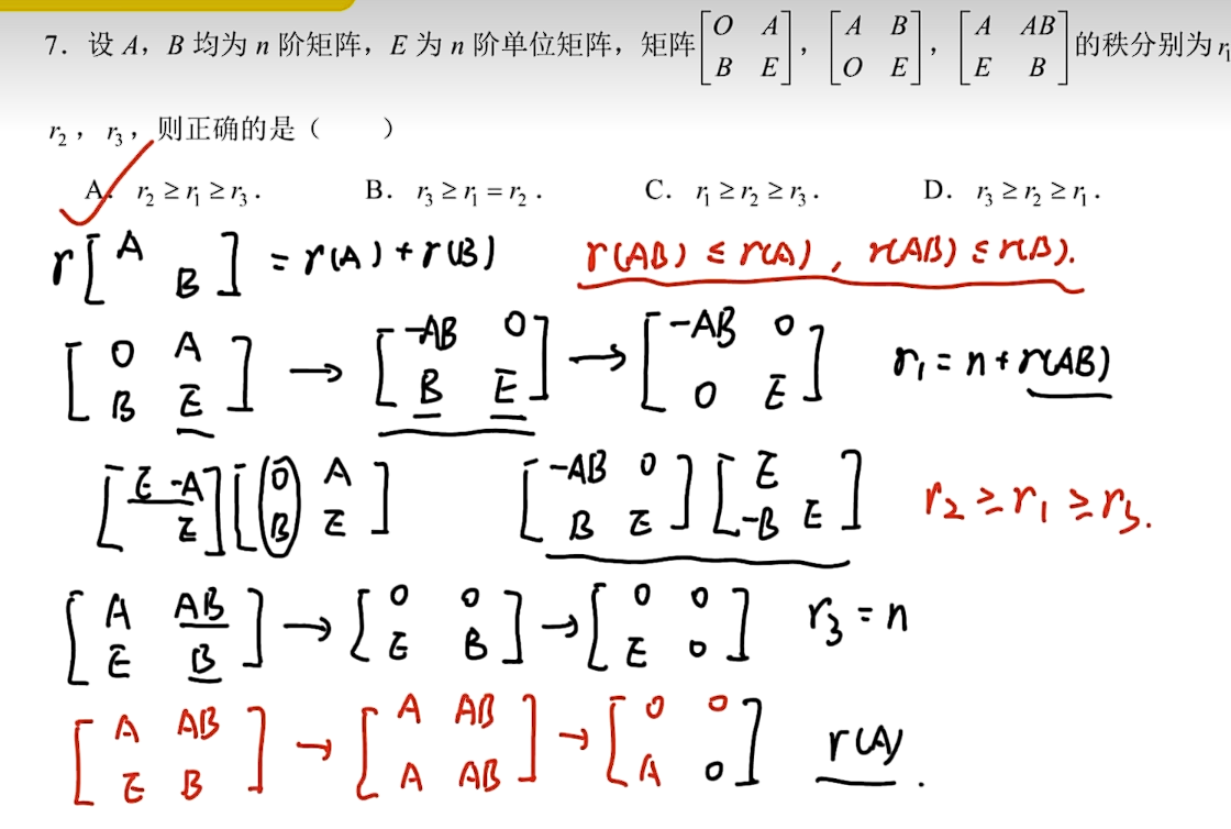
Comments