408 Exam Notes: Data Structures, Computer Organization, OS, and Networks
Sep 9, 2026128 min
Complete revision notes for data structures, computer organization, operating-system scenarios, and computer networks.
These notes organize concepts, examples, derivations, and revision reminders by topic, with the original figures. Apply each result under its stated assumptions and the model and data specified by the exercise.
Data Structures
Linked lists
Disjoint-set union (code, optimization operations, and visualization of root merging)
Implementations of Prim’s and Dijkstra’s algorithms without priority queues
Simulation of orthogonal lists and adjacency multilists (be able to draw them)
Heap implementation code, and code that uses a heap to implement a priority queue
Red-black trees (definitions and conclusions, insertion and deletion)
Loser trees and replacement selection (loser tree + sequence numbers), the role of loser trees in merging, and the depth of a loser tree
Computer Organization
Special floating-point values and flag generation
The principles and circuits of multiplication and division, the number of shifts in Booth multiplication and division, and rounding
The procedure-call process, stack frames, and their respective responsibilities
Multiprocessors and modern processors
A comprehensive summary of the single-cycle datapath in Yuan’s textbook
Operating Systems
Interprocess communication methods
Simplifying resource-allocation graphs and determining the conditions for deadlock
Virtual machines and the detailed SPOOLing process
File-system mounting
Bitmaps and the grouped linked-list method
Multiprocessor scheduling
Wear leveling
Computer Networks
The roles of, and differences between, the layers of OSI and TCP/IP
Physical-layer line coding for digital data, such as Manchester encoding; distinguish this from analog-signal modulation.
PPP and P2P protocols
Virtual circuits
OSPF, BGP, and DHCP messages and their specific addresses
The IP multicast process and IGMP
Hamming-code checking and error correction
Reservation-time calculations and NAV-value calculations in 802.11
Mobile IP
Data Structures
Things to remember: the various implementation procedures for external sorting; the three types of threaded binary trees; the applicability, purposes, and drawing methods of orthogonal lists and adjacency multilists; be able to write out the complete manual calculation processes for Dijkstra’s algorithm and the critical path; insertion and deletion in balanced trees, red-black trees, and B-trees; loser-tree sequence numbers and their use in replacement-selection sorting
Stacks and Queues
In linked queues and stacks, insertion and deletion update node links as well as the appropriate front, rear, or stack-top pointers. Inserting into an empty queue normally initializes both front and rear. After deleting the last data node, restore the empty-queue pointer state: without a sentinel, both front and rear are NULL; with a sentinel, the rear normally points back to it. Stack insertion and deletion operate at the top.
The logic of a prefix expression is simply the reverse of a postfix expression: a postfix expression is converted from left to right, and a prefix expression is exactly the opposite. Here is a manual calculation example for ${((1 + 2) * 3) - (4 + 2)}$: work from left to right and from the inside outward, moving the operators to the front. ${(1+2)}$ becomes ${(+12)*3}$; then handle the right-hand side, ${(4+2) \Rightarrow (+42)}$. Thus, ${((+12)*3)-(+42)\Rightarrow (*+123)-(+42)\Rightarrow -*+123+42}$. For a computer program, the steps are as follows:
Reverse the infix expression.
Replace every left parenthesis ( with a right parenthesis ), and every right parenthesis ) with a left parenthesis (.
Apply the infix-to-postfix algorithm to the reversed token sequence, using a stack for operators. Reverse the handling of associativity for equal-precedence operators as well; do not reuse the usual pop condition unchanged. Treat each multidigit number as a single token.
Reverse the final result again to obtain the prefix expression.
For both prefix and postfix expressions, the idea for conversion to infix is the same: use a stack to hold operands, and pop them in sequence when an operator is encountered. Simulate a postfix expression from left to right, or a prefix expression from right to left.
Tree Structures
Tree Structure
Let the maximum degree in a tree be ${max_d}$. The total number of nodes is then ${\displaystyle n=\sum_{i=0}^{max_d}n_i=\sum_{i=1}^{max_d}i\times n_i+1}$. Note that the two lower summation indices differ.
Binary Trees
For a binary search tree with distinct keys, inorder traversal produces a strictly increasing sequence. A fixed set of keys fixes that sequence, but inorder alone does not determine the tree shape. Unlabeled binary trees with $n$ nodes have $C_n=\frac1{n+1}C_{2n}^{n}$ distinct shapes. If the nodes have distinct labels and different label assignments count as different trees, there are $C_n n!$ trees. These formulas count tree shapes or labeled trees. With distinct node identifiers, preorder or postorder together with inorder uniquely determines the tree.
When a tree with ${n}$ nodes is converted into a binary tree, its ${w=n-1}$ edges are divided into left pointers and right pointers. A left pointer points to a child, and a right pointer points to a sibling, giving the following properties:
Number of left pointers: each nonleaf node retains one left pointer to its first child, so the number of left pointers equals the number of nonleaf nodes.
Number of right pointers: the remaining edges represent sibling relationships, that is, right pointers.
Converting an ordered tree with $n$ nodes to a left-child/right-sibling binary tree leaves the root without a right subtree because it has no siblings. The remaining $n-1$ nodes form its left subtree, giving $C_{n-1}$ shapes. The subtraction removes the root from the node count; tree height is not the argument of the Catalan formula.
When a forest is converted into a binary tree, if the forest has ${n}$ nonterminal nodes, the corresponding binary tree should have ${n+1}$ nodes without a right child. Proof: among ${x}$ root nodes, the rightmost root certainly has no right child. For each of the ${n}$ nonterminal nodes, similarly to the roots, its children include a rightmost child without a sibling node, giving a total of ${n+1}$.
An inorder traversal of a binary search tree produces an ascending sequence (not a preorder traversal).
A binary search tree is searched by comparing nodes one at a time. Count the nodes visited along the path, rather than the tree’s height or the path length.
The path length of a tree is defined as the sum of the lengths from the root to all nodes. To minimize the tree’s path length, every node moves upward as far as possible, which happens to satisfy the definition of a complete binary tree. Therefore, a complete binary tree has the minimum path length.
In a binary tree, B-tree, and so on, a node’s predecessor should be the rightmost node in its left subtree. However, the node may have no left subtree; in that case, return to the parent to look for the predecessor or successor.
Threaded binary trees
A nonempty binary linked tree with $n$ nodes has $2n$ child-pointer fields. Its $n-1$ real edges use that many fields, leaving $2n-(n-1)=n+1$ null fields. These fields may become threads: a null left pointer points to the predecessor and a null right pointer to the successor. In a nonempty inorder-threaded tree without an extra sentinel, the first node has no predecessor and the last has no successor, giving $2$ null threads and $n-1$ nonnull threads. For preorder or postorder threading, the endpoint nodes may already have real child pointers, so count according to the actual structure.
A threaded binary tree uses a binary linked structure and is built by traversing in the chosen order. If a node lacks a left child, use the left pointer as a predecessor thread; if it lacks a right child, use the right pointer as a successor thread. Tags distinguish threads from real child pointers.
Find predecessors and successors in preorder-, inorder-, or postorder-threaded trees according to the corresponding traversal. In postorder, an existing successor thread in an otherwise null right pointer gives the successor directly. If the right pointer is a real child link, parent information is generally needed. The successor may be the parent or the first postorder node in the parent’s right subtree; that first node cannot always be found by following left links alone. A ternary linked structure stores left-child, right-child, and parent pointers, making general postorder-successor handling easier. A binary-link implementation may instead need a stack or a search from the root to find the parent.
Binary-search decision trees
To calculate successful binary-search lengths, build the binary-search decision tree for the sequence positions. A node’s comparison count is its level measured from the root, with the root at level 1. Weight these counts by the search probabilities when computing the average successful search length.
Binary-search decision trees have a consistent shape: if a binary search goes as far left as possible, the left subtree takes priority; otherwise, the right subtree takes priority. The two cases cannot coexist.
Balanced Search Trees (AVL, Red-Black, B-Trees, and B+ Trees)
AVL Trees
In a balanced binary tree, the balance factor is the height difference between the left and right subtrees. Thus, the minimum number of nodes that can form a balanced binary tree is obtained when every nonleaf node has a balance factor of 1. In terms of height, the formula is ${C_n = C_{n-1}+C_{n-2}+1}$, where ${C_0=0,\,C_1=1,\,C_2=2}$. The maximum number of nodes is that of a perfect binary tree. Question: the maximum depth of a balanced binary tree with 16 nodes: since ${C_5=12 \lt 16 \lt C_6=20}$, it is 5.
Deleting a node from a balanced tree and then adding it again may produce the original tree because the tree can rebalance itself. However, a binary search tree has no balance requirement, so if the deleted node is not a leaf, the resulting tree must differ from the original tree.
Given any sequence, to determine the number of different balanced binary trees, choose nodes around the middle as the root, because the sizes of the left and right subtrees need to be balanced. Then discuss these root choices separately. Once a root is fixed, recursively determine its left and right subtrees in the same way. Consider this example: The number of balanced binary trees that can be determined by the sequence {1, 4, 5, 10, 16, 17, 21}. First, the self-balancing requirement gives the candidate root set {5, 10, 16}. By symmetry, 5 and 16 are symmetric. Consider 5: its left subtree is fixed as 1, 4, with two possibilities; the right subtree has a maximum height of 3 and candidate roots 16, 17, with four possibilities, giving ${2\times 4=8}$ possibilities in total. Next consider root 10: both subtrees have a size of 3. Because a balanced tree of height 2 has at least 2 nodes and one of height 3 has at least 4 nodes, each subtree has only one possibility. Thus, the total is ${8+8+1=17}$.
B-Trees and B+ Trees
Insertion and deletion in B-trees
Insertion: a nonroot node of an order-$m$ B-tree has at least $\lceil m/2\rceil-1$ and at most $m-1$ keys; a nonempty root has at least one key. A common algorithm first inserts the new key into the appropriate leaf. If that node temporarily has $m$ keys, promote key $\lceil m/2\rceil$ to the parent and leave the keys on either side in two nodes. The promoted key becomes a separator in the parent; a new root is created only when the root splits. If the parent overflows, continue splitting upward recursively. Specify the rounding convention when selecting the middle position.
Deletion: be sure to note that deletion replaces the current node with a leaf node (terminal node). That is, if the node being deleted is not a leaf, find its predecessor or successor, replace it, and then delete after replacement. Thus, the actual deletion is essentially from a leaf. See the Wangdao textbook for details. There are three cases: direct deletion, borrowing from a left or right sibling with enough keys, and merging a sibling with the parent.
Here is an additional example in which the siblings do not have enough keys to lend:
Original note figure 1
Since 71 is a leaf node, delete it directly, leaving an empty node. Then inspect the left sibling (55) to see whether it has enough keys to lend. It does not, so merge the parent and the left sibling into a leaf node. The parent is now empty, so inspect its left sibling (20) to see whether it has enough keys to lend. It does not, so merge the parent and the left sibling. The resulting root is 20,47, with three children: [18],[23],[55, 60].
A fixed-length code set converts data into binary strings of a fixed length, so the binary tree it forms is fixed, and every data item is at a leaf node.
Heaps
The number of comparisons during heap insertion and deletion
During insertion, insert directly at the rightmost leaf position and then adjust the heap: starting from this node, compare it with its parent in sequence and swap if it is larger. Since the original heap property remains, no other comparisons are needed.
During deletion, first delete the root, and then let the rightmost leaf replace it as the root. Adjust the heap as follows: starting from the root, first compare the values of its two children, select the extreme value, and compare the root with it. Continue until the root no longer swaps downward.
If an initial sequence must be adjusted into a heap, work backward starting from the last nonleaf node.
Loser Trees (Tournament Trees)
Loser trees (tournament trees)
Loser trees are suitable for multiway merging, so first use an external-selection algorithm to choose the initial merge runs, and then construct the loser tree. Suppose internal sorting of the initial file produces four initial merge runs: {6,8}; {3,9}; {1, 5}; {2, 7}. The loser-tree construction process is as follows.
Original note figure 2
A loser tree is a complete binary tree. Its root points to the smallest number, and its nodes store merge-run numbers.
As the figure shows, a ${k}$-way loser tree has depth ${\lceil log_2k \rceil+1}$, but its height is ${\lceil log_2k \rceil}$ (excluding the champion node and leaf nodes), independent of the number of nodes.
A loser tree selects the current smallest record each time. Updating it takes a number of comparisons corresponding to its height, typically about $\log_2 k$. Increasing the merge fan-in $k$ increases the height and per-update comparisons but can reduce the number of merge passes and disk I/O, often improving external sorting when memory permits. Total comparisons also depend on the total number of records, merge passes, and fan-in used in each pass; calculate them from the actual merge process.
A loser tree can optimize the generation of initial merge runs, that is, improve replacement-selection sorting by selecting MINMAX more quickly.
The records in the in-memory workspace serve as the loser tree’s external nodes, while the parent of the loser tree’s root points to the record with the smallest key in the workspace.
To make it easier to select the MINIMAX record, attach a merge-run sequence number to each record. When comparing keys, compare run numbers first: the record with the smaller run number wins; if the run numbers match, the record with the smaller key wins.
Construction of the loser tree can begin by setting the run numbers of all workspace records to 0. Then, as w records are read from FI into the workspace one by one, adjust the loser tree from top to bottom. Since these records have run number “1,” they all lose to records with run number 0, thereby filling the loser tree’s nodes one by one.
Original note figure 3
(Multiway) Huffman Trees and Code Sets
To determine the number of empty nodes that must be added in a multiway Huffman tree or multiway merge, consider the following algorithm. Consider an optimal merge tree with ${n}$ nodes and a fan-in of ${k}$. Suppose a strict ${k}$-ary tree has ${n_0}$ leaf nodes and ${n_k}$ nodes of degree ${k}$. Then ${n=n_0+n_k=k\times n_k + 1}$. Eliminating ${n}$ gives ${n_0=(k-1)n_k+1\Rightarrow n_k=(n_0-1)/(k-1)}$. Let ${(n_0-1)\mod(k-1)=x}$. If ${x=0}$, a ${k}$-ary merge can be constructed; otherwise, there are ${x}$ extra nodes. We know that ${x\lt k}$, so let these ${x}$ nodes form a new merge run. However, this requires one additional node to be the combined node for ${\sum x}$. Therefore, only ${k-x-1}$ new nodes need to be added, with one node lying internally and having degree ${k}$.
For multiway balanced merge sorting of ${\displaystyle n}$ records, the number of merge passes depends on the chosen merge fan-in. Here, one record is one merge run. If the given number of merge passes is ${\displaystyle k}$, the selected fan-in must satisfy ${\displaystyle k- 1\lt \lceil log_{d}(n) \rceil \leq k}$. For example, if ${\displaystyle 149}$ records undergo only 4 passes of multiway balanced merging, the valid fan-ins are ${\displaystyle 4,\,5}$, whereas ${\displaystyle \lceil log_{6}(149) \rceil =3}$.
Graph Structures
In an undirected graph, each node’s degree is its number of incident edges, so the total degree of the graph is twice the number of edges. In a directed graph, each node’s degree is the sum of its outdegree and indegree.
An adjacency matrix is suitable for dense graphs, frequent queries of “does an edge exist between any two vertices?”, and adding or removing edges. An adjacency list is suitable for sparse graphs and frequently traversing neighbors or the entire graph. Many algorithms use adjacency lists, such as DFS, BFS, Prim, Kruskal, and topological sort.
For an adjacency matrix $A$ whose entries indicate edges or count parallel edges, $A^n[i][j]$ is the number of walks of length $n$ from vertex $i$ to vertex $j$. Walks may repeat vertices and edges. Matrix powers do not directly count simple paths, which forbid repeated vertices.
Prim’s algorithm has time complexity ${O(n^2)}$, independent of the number of edges, and is suitable for dense graphs. Kruskal’s algorithm has time complexity ${O(m\times log_2m)}$, independent of the number of vertices, and is suitable for graphs with sparse edges and many vertices.
Searching
Hashing
The average unsuccessful-search length for a hash table depends on its hash function. For example, if the array length is 10 and the hash function uses modulus 7, calculate the unsuccessful-search lengths for indices 0–6 only; do not include the later positions.
When calculating unsuccessful hash-search lengths, with separate chaining, search only the pointers that have values; the next null pointer is not counted as a comparison. With probing, if the current position is the last occupied position and the next position is empty, the next position is also counted as a search.
When calculating the load factor for separate chaining in a hash table, the count of nodes loaded into the hash table must include all the pointers. That is, if the linked list corresponding to 2 has size 2, both nodes count toward the load factor’s numerator.
Strings and Miscellaneous Topics
When merging two sorted sequences, the worst-case number of comparisons is O(m + n - 1).
When calculating the KMP algorithm using my method, array indices start at 1, so position 0 is the beginning (that is, nothing is there; move the entire segment forward). When the corresponding next-array value is 0, move the entire segment forward and then perform i+1, that is, j=next[j], i++, j++. Note: when constructing the next array, the head and tail must not lie within the same substring. For aaaab, the next value of b should be 4, that is, a|aaa = 3 + 1.
A multiway linked structure uses several pointer fields for different link relationships. A binary linked structure has two pointer fields and a ternary linked structure has three; their precise meanings depend on the data structure.
Sparse matrices
Compressing a sparse matrix uses triples and necessarily loses random-access capability.
Transposing a sparse matrix A[m][n] stored as triples requires at least three steps: (1) swap the matrix’s row and column values; (2) swap i and j in every triple; (3) reorder the triples to complete the transpose, because the triples are arranged primarily in row order.
In quicksort, if a pass is defined as processing all elements once, the following cases determine whether the current sequence could be the result of the second pass:
If the pivot processed in the first pass is at the beginning or end (that is, the maximum or minimum), this pass fixes one final position. In the second pass, only one side can be chosen, fixing one more final position. There are then two final positions.
If the pivot is not at the beginning or end, three final positions are fixed.
Computer Organization
Things to remember
The various special cases of IEEE754 floating-point numbers; the conceptual part of ISA; parallel-processing techniques and multicore-processing concepts; the ranges of the various internal computer number representations; biased representation and the concept of machine zero in floating-point numbers; specific floating-point operations, exponent alignment, rounding, and so on; the basic concepts of multiprocessors; the scope of ISA
Computer Architecture
CPI is the number of clock cycles required by one instruction. It reflects how many cycles the instruction needs to run on the hardware (because registers and so on can only be used once in each clock cycle), so CPI is independent of the clock period.
When calculating the size of an entire program segment, the question generally gives the complete code segment. Calculate from its first line, the starting address ${A}$, and its last line, the ending address ${B}$. Note here that the ending address of the last line is not the starting address of the last instruction, but the starting address of that instruction + the instruction length. If the last instruction is ${x}$ addressable units long, then ${Lenth=B+x-A\,\,\text{or}\,\,B+x-1-A+1}$.
General-purpose registers store operands and various addresses. Their width is determined by the machine word length; word length/machine word length is the width of the datapath.
According to the principles of the von Neumann computer architecture:
Instructions and data are stored in the same memory and have the same format; they are not physically separated.
The CPU fetches instructions from memory at the address specified by the program counter (PC).
Data is accessed through the address fields in instructions.
Instructions and data are distinguished mainly because the CPU accesses memory in different phases of the instruction cycle: the instruction-fetch phase accesses instructions, while the execution phase accesses data.
Differences and relationships among word length, machine word length, instruction length, and memory word length
Word length: the number of bits a processor naturally handles in one operation, usually related to general-purpose register and ALU widths. External data-bus width, MDR width, and machine word length need not be identical; determine each from the specified datapath and memory interface.
Machine word length: the processor’s natural arithmetic width, commonly associated with general-purpose registers, the ALU, and major internal datapaths. It need not equal the external data-bus or MDR width.
Instruction length: the number of bits in an instruction’s encoding. In an exercise model that fetches whole words, reads one memory word per access, and excludes overlapping accesses, an instruction twice the memory word length requires two accesses; equal lengths require one. Whether one access equals one machine cycle depends on the specified machine. Real ISAs may use byte-based or variable-length encodings, and one read may cover several instructions or part of one.
Memory word length: the number of bits in one memory word as defined by the machine model. If the MDR holds one full-word access, its width matches that word; the addressing unit may still differ from the full-word access width. Equality or integer-multiple relationships with machine and instruction lengths depend on the particular organization.
A main-memory address identifies an addressable unit. Its width depends on the number of such units and must be distinguished from data word length. MAR must cover the machine’s supported address space; alignment of individual data objects is a separate issue.
Calculate CPI by definition: $\mathrm{CPI}=\text{total clock cycles}/\text{completed instructions}$, the average cycles per instruction. Instructions completed per clock cycle are measured by IPC; with the same accounting scope, $\mathrm{IPC}=1/\mathrm{CPI}$.
Data Representation and Computation
With the same number of bits, biased representation and two’s-complement representation have the same representable range.
When calculating the extreme values of floating-point numbers, pay particular attention to those special cases, such as an all-1 exponent or an all-0 exponent. This part must be memorized.
The purposes and meanings of flags in the PSW
CF is the carry/borrow flag and is used for unsigned range checks. Under the convention $CF=Sub\oplus C_{out}$, addition has $Sub=0$, so CF equals the adder’s carry-out $C_{out}$; both are 0 when there is no carry. Subtraction uses $A+\overline B+1$ with $Sub=1$: if unsigned $A\ge B$, then $C_{out}=1,\ CF=0$ and there is no borrow; if $A\lt B$, then $C_{out}=0,\ CF=1$ and a borrow occurs. Signed overflow is determined separately by OF and must not be confused with carry or borrow.
OF is the overflow flag and is meaningful only for signed numbers. ${OF=C_n \oplus C_{n-1}}$: a signed-number operation overflows if the carries associated with the sign bit and the highest numerical bit differ.
SF is the sign bit, the most significant bit of the number, and is meaningful only for signed numbers.
ZF is the zero flag and is meaningful for both.
Unsigned comparisons primarily use ZF and CF; SF and OF do not directly determine the result. With CF set to 1 on a subtraction borrow, $A-B$ has no borrow when $CF=0$, including $A=B$. Strictly greater also requires $ZF=0$, so $\overline{ZF+CF}=1$ means unsigned $A\gt B$, where the plus sign denotes logical OR.
Cast operators have higher precedence than multiplication and division, so (float)(x+y)/2 follows x+y -> (float)(x+y) -> /2. For mixed types, apply integer promotions and the usual arithmetic conversions: for example, arithmetic between float and int normally converts the int to float. A signed/unsigned mixture also depends on rank and representable ranges; its result is not always unsigned. In the common model with 16-bit short, 32-bit int, and two’s complement, converting a negative short to unsigned int can produce the bit pattern of sign extension, while converting unsigned short to an int that represents its entire range corresponds to zero extension. Check the source type and value range before extending a shorter type. A cast normally performs a value conversion; integer-to-floating conversion may also round, so casting is not always a reinterpretation of unchanged bits. Evaluate the following code under that common width and two’s-complement conversion model.
Suppose a Hamming code has ${k}$ parity bits and ${n}$ data bits. Then ${k}$ must satisfy ${2^k \geq n+k+1}$. The sender must then convert the data into Hamming-code format. Using 1001011 as an example, ${k=4}$ parity bits are needed, for 11 transmitted bits in total.
Hamming parity bits conventionally occupy positions $2^i$, namely $1,2,4,8$. With even parity, the parity bit at position $2^i$ is the XOR of the data bits in its group; the corresponding binary-index bit is 1 at every position in that group. For the data positions $3,5,6,7,9,10,11$ in this example, $a_1=a_3\oplus a_5\oplus a_7\oplus a_9\oplus a_{11}=1$ and $a_2=a_3\oplus a_6\oplus a_7\oplus a_{10}\oplus a_{11}=0$. Position 11 has binary index 1011 and therefore also belongs to the second parity group. Similarly, $a_4=1,\ a_8=0$, producing codeword 10110010011.
The receiver XORs all bits in each check group, including that group’s parity bit, to obtain syndrome bits $h_i$. For received word 10110110011, $h_1=a_3\oplus a_5\oplus a_7\oplus a_9\oplus a_{11}\oplus a_1=0$ and $h_2=a_3\oplus a_6\oplus a_7\oplus a_{10}\oplus a_{11}\oplus a_2=1$; similarly, $h_4=1,\ h_8=0$. Ordered as $h_8h_4h_2h_1$, the syndrome is 0110. Assuming at most one erroneous bit, invert bit six. A syndrome of 0000 means no error was detected: it implies no error under the single-error assumption, but some multiple-bit errors can also have zero syndrome.
A machine can represent an exact zero and can also round a sufficiently tiny result to zero. In floating-point arithmetic, distinguish zero, subnormal values, and underflow. In a traditional format an actual zero significand represents zero; IEEE 754 defines positive and negative zero using an all-zero exponent field and fraction field, with the sign bit distinguishing them. A normalized number whose stored fraction is zero still has an implicit leading 1 and is normally nonzero. Underflow may produce a subnormal value or a rounded zero. Biased notation encodes exponents using an offset, but whether an all-zero bit pattern represents zero is a property of the format, not a consequence of biased exponents alone.
The numerical range of IEEE 754 floating-point numbers
A normalized number’s exponent field is neither all zeros nor all ones. With $k$ exponent bits, $p$ stored fraction bits, and $\mathrm{bias}=2^{k-1}-1$, the smallest positive normal value is $1.0\times2^{1-\mathrm{bias}}$ and the largest is $(2-2^{-p})\,2^{\,2^{k-1}-1}$. Here $p$ excludes the implicit leading bit of a normalized significand.
A subnormal value has an all-zero exponent field and a nonzero fraction, without an implicit leading 1. Its smallest positive value is $2^{1-\mathrm{bias}-p}$, corresponding to fraction 0.00…01. The stored fraction widths are $p=23,52$ for binary32 and binary64; normalized precision including the implicit bit is 24 and 53 bits, respectively.
Floating-point rounding distinguishes rounding toward zero, toward positive infinity, toward negative infinity, and to nearest. IEEE 754’s default nearest mode is “round to nearest, ties to even.” Compare the entire discarded portion with half a unit at the retained precision: round upward in significand magnitude when it is larger, truncate when it is smaller, and at an exact tie choose a retained least significant bit of 0. Thus the first discarded bit alone is insufficient; later nonzero bits and the parity of the retained result also matter.
An operation on two normalized floating-point numbers can produce a subnormal number. For example, if ${\displaystyle A=0x00800001,\,B=0x80800000}$, then ${\displaystyle A+B=0x00000001}$.
Adders, multipliers, and dividers
For subtraction of either signed or unsigned numbers, in x-y, feed x unchanged into one side of the adder, bitwise invert y for the other side, and set sub to 1.
Whether the ALU adds the partial product and the multiplicand is determined by the multiplier’s least significant bit (0: do nothing; 1: add).
When shifting during sign-magnitude multiplication, perform a logical right shift on the carry bit, partial product, and product portion together.
A fast array multiplier does not contain a shifter.
${\displaystyle n}$-bit multiplication and division require approximately ${\displaystyle n}$ addition/subtraction operations and ${\displaystyle n}$ shift operations. Remember the single XOR operation on the sign bits.
Memory Systems
Memory Classification and Functions
The classifications and purposes of various memories
Random-access memory (RAM, volatile); read-only memory (ROM, also supports random access, and writing is slower than reading); sequential-access memory (magnetic tape, supports only sequential access); direct-access memory (magnetic disks and optical discs, whose access process includes both random access, to locate a track, and sequential access, to locate a sector).
Static memory (SRAM, higher power consumption, nondestructive readout, no refresh required); dynamic memory (DRAM, lower power consumption, destructive readout, regeneration required after reading, only for the cells read, and periodic data refresh by row to prevent data loss).
Main memory is implemented using RAM and ROM; control memory (in microprogramming) is implemented using ROM.
The width of the memory address register MAR depends on the number of addressable units, so both capacity and addressing unit are required. For 128 KB addressed in 16-bit, 2 B words, there are $128\mathrm{KB}/2\mathrm B=2^{16}$ addressable units, requiring at least 16 MAR bits. Byte addressing requires 17 bits. A 16-bit machine word alone does not specify the addressing unit; dividing capacity by unit size yields a unit count.
Under a specified size-based alignment rule, an object’s byte address must be a multiple of its type size. For example, in a model with 2 B short and 4 B int, use 2-byte and 4-byte alignment, inserting padding when necessary. Type sizes, alignment requirements, and floating-point encodings depend on the target ABI and the exercise. These common widths and IEEE 754 conventions are not universal guarantees of the C language.
A main-memory address consists of a main-memory block number + an offset within the block. The block number maps to the cache’s ${tag}$ + cache-set-number fields, and the offset is the same.
The memory cycle is the minimum interval between the starts of two independent accesses to the same bank, reflecting access and recovery constraints. Determine from the specified timing whether data preparation, internal recovery, and external bus transfer are separate or overlap. Do not categorically exclude transfer time or add time that has already been counted.
DRAM refresh
DRAM activates rows and restores their stored charge. Sense amplifiers and related static holding circuits retain the activated row as the row buffer. In an organization that activates a whole row, buffer capacity equals the number of data bits in that row; it need not be a separate SRAM memory array.
DRAM normally receives refresh commands from the memory controller and refreshes the selected rows internally. In self-refresh mode, the chip schedules refreshes autonomously. Refresh is usually transparent to the CPU, which does not imply independence from external control. Read regeneration is also normally automatic hardware behavior and concerns the cells just read; periodic refresh ensures that all retained data is refreshed in time.
Refresh operates by row and does not need a column address to select an individual word in the row. Row numbers may come from external inputs or an internal refresh counter; refresh commands, chip selection, and bank selection still follow the device’s protocol.
If a parallel chip group can refresh the corresponding row of every equal-sized chip simultaneously, its number of row-refresh rounds equals one chip’s row count, and total time is rounds times time per round. If a controller schedules banks, ranks, or chip groups separately, or concurrency is constrained, use that actual schedule. Chip count alone does not imply fully parallel refresh with unchanged elapsed time.
Here is a comprehensive example: There are 16 DRAM chips, each 1M X 4 bits. Every pair of chips is combined by width expansion into a 1M X 8-bit memory bank. These banks use low-order interleaving to form an 8MB memory. The memory is byte-addressable and connected to a 64-bit memory bus. Main memory can read or write at most 64 bits at a time, and its memory cycle is 1ns.:
For each 1M x 4-bit DRAM chip, assume 10 row-address bits and 10 column-address bits in this example, giving 1024 rows and 1024 columns; capacity alone does not uniquely determine that split. Given a row number, all the corresponding row’s data is read into the chip’s row-buffer register. The number of entries in the row buffer equals the number of columns, and each entry is 4 bits wide. Thus, one chip’s row-buffer register has size ${\displaystyle 1024 \times 4bit}$, and the total row-buffer size for the memory is ${\displaystyle 1024*4*16/8=8192B}$. The buffer capacity here follows the stated row organization and the associated static holding circuits, such as sense amplifiers.
The memory is byte-addressable, meaning that each byte corresponds to one memory location. One chip supplies 4 bits of data, so selecting one memory location means selecting one location in a memory bank. Selecting a location in a bank simultaneously selects the 4-bit locations at the same address in two DRAM chips, which output together onto 8 data lines of the memory bus. Width expansion does not change the number of memory locations; it increases the size of each location. The number of addresses stays the same, while the data width corresponding to each address increases. Depth expansion does not change the size of a location; it increases the number of locations and the number of address indices, while the amount of data corresponding to each address remains unchanged.
DRAM multiplexes row and column address pins. This example needs 10 address pins and 4 data pins, totaling $10+4=14$; control, power, and other pins are additional.
A double variable x has main-memory address 01 2345H. The bus is 64 bits wide. With simultaneous activation, 8 banks are activated in one memory cycle, each supplying 1B of data. Because low-order interleaving is used, the main-memory address consists of a 20bit within-block address + a 3bit block number. Thus, the first 20 address bits of these 8B are the same, and the final three address bits range from 000 to 111, representing the 8 banks. The low three bits of x’s address are 101. The first simultaneous activation obtains the 8B from 01 2340H through 01 2347H, of which 01 2345H through 01 2347H are x’s first three bytes. The second memory cycle obtains the 8B from 01 2348H through 01 234FH, and 01 2348H through 01 234CH are x’s final five bytes. Reading x therefore requires two memory cycles.
In the stated model where corresponding rows of all chips can refresh simultaneously and each refresh takes one 1 ns memory cycle, count the 1024 rows of one chip: refreshing all rows occupies $1024\mathrm{ns}$ in total. Concentrated refresh makes this dead time continuous, while asynchronously scheduling row refreshes distributes it. Every refresh period must cover all rows. If a refresh period of $20480\mathrm{ns}$ is additionally specified, the dead-time fraction is $1024/20480=5\%$. The stated 1 ns memory cycle alone does not determine that percentage.
Calculating the numbers of pins and chips for SRAM and DRAM
A chip organized as 8M × 8 bits has $2^{23}$ locations of 8 bits each, for 8 MB total capacity. Separate address pins require 23 lines and data pins require 8, totaling $23+8=31$. DRAM can split the 23-bit address into 11 row bits and 12 column bits and multiplex them over 12 address pins in two transfers; fewer rows can reduce the number of row refreshes. Address plus data pins then total $12+8=20$. These totals exclude chip-select, read/write, clock, power, and other pins.
If the required number of RAM chips is asked for, first observe the computer’s addressing unit, then calculate the required total address-space size and the size of one RAM chip, divide the former by the latter, and round upward.
Here is an example of expansion in both dimensions: “Several 8K x 8-bit chips form a 32K x 32-bit memory. The memory word length is 32 bits, and memory is word-addressable. Find the highest address in the chip containing address 41F0H." First perform width expansion: 4 chips form an 8K x 32-bit unit, connected directly to the data lines without chip selection. Then perform depth expansion: clearly, 4 groups of the width-expanded chips are required, so use the high 2 bits for chip selection. Each group represents ${8K=2^{13}}$, that is, a 13-bit address space. Thus, bits ${1 \sim 13}$ represent the address space, and bits ${14 \sim 15}$ select the chip. Since ${41F0H=010|0...}$, the corresponding highest address is ${010|1FFFH =5FFFH}$.
One bus transaction includes:
Sending the starting address and command
Memory prepares or reads data. Denote first-item preparation time by $T_{\mathrm{prep}}$ and obtain it from the access timing; equate it to one memory cycle only in a model that explicitly does so.
Placing the data on the data bus for transfer
In the pipelined preparation model for multimodule interleaved memory, transmit the starting address and command, wait for the first data item to become ready, then transfer the items successively. If address/command transmission takes one bus period $T_{\mathrm{bus}}$, first-item preparation takes $T_{\mathrm{prep}}$, and the bus then transfers one item per period for $n$ transfers, total time is $T_{\mathrm{bus}}+T_{\mathrm{prep}}+nT_{\mathrm{bus}}$. Substitute one memory cycle for first-item preparation only when specified. Here $n$ counts transfers, or words when one word is sent per transfer; a multi-bit bus normally sends several bits per cycle.
Original note figure 4
Low-order interleaving in multimodule memory has two activation methods: staggered activation and simultaneous activation.
Multibank parallel memory has multiple modules, each with its own memory bank, MAR, MDR, and read/write/control circuits. Each module is an independent memory.
When the number of bits transferred by each module equals the data-bus width, staggered activation is used. Its storage process was described in the earlier discussion of a bus transaction. Let the memory cycle be ${T}$ and the bus cycle be ${r}$. The number of modules must be at least ${m=T/r}$. One datum can be read or written every ${1/m}$ memory cycle, and conflicts may occur during this process.
When the combined data width of a simultaneously activated group equals the bus width, the modules can form one parallel bus transfer. Misalignment may fetch unused bytes. For example, four DRAM modules specified as 64KB × 4 bits provide only 16 bits, so pairing that statement with a 32-bit bus is insufficient to conclude that one parallel transfer fills the bus; the organization must be clarified. To illustrate 32-bit simultaneous activation using four byte-organized 8-bit modules, fetching an 8 B double starting at …AH, whose low two bits are 10, accesses three groups: [00,01,10,11]; [00,01,10,11]; [00,01,10,11]. The useful bytes are 10 and 11 of the first group, all four bytes of the second, and 00 and 01 of the third. The other four fetched bytes are not part of the requested value.
Multibank interleaved memory may encounter bank conflicts during access. For example, with 4-way interleaved memory, the CPU’s main-memory address sequence is 03,09,11,02,33,25,0D,04,08,29,43,0A (all hexadecimal). Ideally, one datum can be read or written every 1/4 cycle; call that time 𝛥𝑡. The addresses in each memory module are determined by the final two binary address bits: module 0: 00, 04, 08, 0C, 10; module 1: 01, 05, 09, 0D, 11, 25, 29; module 2: 02, 06, 0A, 0E, 12; module 3: 03, 07, 0B, 0F, 13, 33. Clearly, if the addresses of four consecutive accesses include addresses in the same module, a memory-access conflict occurs. Therefore, 11 and 09, 25 and 11, 0D and 25, 08 and 04, and so on cause conflicts. 29 and 0D also belong to the same module, with an access interval of less than 4𝛥𝑡. However, the conflict when accessing location 08 delays that access by 3𝛥𝑡, which also delays access to location 29 by 3𝛥𝑡. As a result, its access no longer conflicts with access to location 0D.
Because multimodule memory is activated in a pipeline, once steady state is reached, its average transfer speed should be calculated as a pipeline: one bank is transferred per cycle.
Cache
For an instruction, inspect carefully how many accesses actually occur. For example, a[x] = a[x] + 1; a[x] is actually accessed twice here.
Unless otherwise specified, write-through counts as one main-memory access even when the write is placed in a write buffer.
To calculate cache efficiency, first specify the timing model and hit rate $H$. If $T_C$ is hit time and $T_M$ is the complete miss-access time, or the corresponding parallel-lookup model applies, then $T_A=HT_C+(1-H)T_M$. With $r=T_M/T_C$, efficiency is $e=T_C/T_A=1/[H+r(1-H)]$. Compare performance with the no-cache baseline access time $T_{\mathrm{base}}$: $X=T_{\mathrm{base}}/T_A$, reducing to $X=T_M/T_A$ when the model has $T_M=T_{\mathrm{base}}$. If the cache is checked first and a miss then incurs an additional $T_M$ main-memory access, use $T_A=T_C+(1-H)T_M$; include the initial lookup.
Main memory and cache each have an independent address space. Cache addresses map to the main-memory address space. Different cache-mapping methods have different cache-address structures:
Direct-mapped cache address: line number + within-block address
Fully associative cache address: line number + within-block address
Set-associative cache address: set number + line number + within-block address
Note: although a cache address contains a set number and line number, the cache structure does not store the set number or line number. It contains a valid bit, tag, data (line length), LRU information (if any), and a dirty bit (if any).
Note: cache capacity means its data-storage capacity, excluding the tag array (tag bits, valid bits, dirty bits, and so on). However, calculations of the total number of cache bits or total cache capacity include the tag array.
Note: the cache’s control fields are the tag array: the valid bit, tag, dirty bit, LRU bits, and so on.
In a $d$-way set-associative cache, the set index selects a set. Typically, $d$ comparators compare its ways’ tags in parallel, using valid bits to determine a hit. One line normally holds one main-memory block. Multiplexing selects the hit way’s data, and the block offset selects the required word or byte within it. Selection widths depend on associativity and within-line organization; a line should not be treated as several main-memory blocks.
Disks
When calculating average disk read/write time, remember that the initial average time until the target sector rotates under the head is half a revolution (do not use this calculation if the question explicitly specifies the head’s initial position). The disk’s data-access rate may not be given explicitly, but it can be derived from the amount of data in one revolution and the time for one revolution.
Track density is the number of tracks per unit length in the radial direction; bit density is the amount of data stored per unit track length. As the radius increases, track density remains unchanged and bit density decreases.
RAID: redundant array of independent disks
RAID0: a disk array with no redundancy and no parity. Striping gives it the fastest read/write speed among RAID levels.
RAID1: a mirrored disk array. Two disks are used as one, improving safety and reliability.
RAID2: uses Hamming-code error correction, improving safety and reliability.
RAID3–5: all use parity, improving safety and reliability.
Instruction Sets and the CPU
Instruction Sets
Instruction Formats
During sequential execution, the PC increment equals instruction length in bytes divided by bytes per addressing unit. Machine word length alone does not specify that unit: on a byte-addressed 16-bit machine, a 2 B instruction advances PC by 2; it advances PC by 1 only when the specified unit is a 2 B word. Branches and jumps update PC according to their target rules.
Enabling/disabling interrupts, changing interrupt masks, accessing protected I/O ports, and modifying memory-management registers or privileged PSW fields are normally privileged operations. User mode generally permits ordinary arithmetic/logic, data transfers, calls, returns, and conditional or unconditional transfers, within authorized resources. Trap or software-interrupt instructions used to enter system calls may be executable in user mode; the ISA and operating system define the exact privilege boundary.
Instruction formats and the corresponding computer encodings
Suppose the computer is a 16-bit computer. With fixed-length opcode encoding, there are half-word instructions (8 bits, common for RR instructions), single-word instructions (16-bit instruction length, with the specific format given by the question), and double-word instructions (32 bits, with the second word generally holding a displacement or effective address).
Common instruction formats are: RR (register–register), RX and RS (register–memory instructions). RX has the format OP R1 X B D, where X is the index register, B the base register, and D the displacement: one register operand R1 and one memory operand, with EA = D+(X)+(B). RS has the format OP R2 R3 B D, that is, two registers and one memory operand, with EA = (B) + D. Other formats are SI (storage–immediate) and SS (storage–storage).
Given this analysis, if a question supplies instructions ${(F0F1)_H(3CD2)_H}$ and ${(2856)_H}$, the first is a double-word instruction and the second a single-word instruction. Their operations can therefore be identified using the instruction formats supplied in the question.
Distinguish fixed/expanding opcodes from fixed/variable instruction lengths. Opcode bits determine the number of encodable operations, not the number of operands per instruction. Expanding opcodes can also fit inside fixed-length instruction words. For example, a 20-bit word with two 8-bit address fields leaves a 4-bit primary opcode. With fixed-length opcodes and two distinct patterns reserved for one-address and zero-address operations, at most $2^4-2=14$ two-address operations remain. With an expanding-opcode scheme that reserves only one primary pattern as a prefix for further one-address/zero-address encodings, at most $2^4-1=15$ two-address operations remain. The two counts depend on the reservation scheme, not merely on whether instruction words are fixed-length.
Both fixed- and variable-length instructions need a PC to track the fetch position. Fixed lengths make sequential increments and boundaries easier to determine, generally simplifying fetching and basic decoding. Variable-length instructions identify boundaries through length information or decoding and may be fetched in blocks and separated in a buffer; fetching a maximum-length region is an implementation choice. Format selection also trades off decoding complexity and code density.
Two kinds of instructions may have implicit operands: zero-address instructions obtain their operands from the top and second-to-top of the stack; one-address instructions obtain an operand from the ACC.
MIPS assembly language and machine language
MIPS is a typical RISC processor: byte-addressable, using 32-bit fixed-length instruction words and fixed-length opcodes. If a given field is 16 bits wide, sign extension or zero extension is required.
Classic 32-bit MIPS has R-, I-, and J-type formats. J-type uses OP(31–26) target(25–0) for pseudo-direct jumps such as J and JAL. If PC denotes the current instruction address, concatenate the high 4 bits of PC+4, the 26-bit target field, and two trailing zeros. This is equivalent to shifting the target field left by 2 before combining the high bits. Four-byte instruction alignment makes the target’s low two bits zero, so they need not be encoded. The PC+4 high bits are particularly important at a 256 MB boundary.
Instruction Cycles and Addressing Modes
One instruction corresponds to one microprogram; that is, both take one instruction cycle.
Displacement addressing depends on the ISA’s base address, sign-extension rule, and displacement unit. A PC-relative branch generally forms its target from the specified PC base plus an extended and scaled displacement. With PC denoting the current instruction address, a classic MIPS conditional branch uses PC + 4 + (sign_extend(imm16) << 2). Indexed addressing normally combines a base, index, and scale to form a data effective address, useful for arrays. Understand it separately from relative branching rather than imposing a universal PC+1+Offset rule.
After an instruction’s execution cycle ends, the processor checks for an interrupt request. If there is one, it enters the interrupt cycle. In that cycle, the CPU performs preparatory work (saving the return point, disabling interrupts, obtaining the interrupt vector, and so on), and then jumps to the interrupt service routine’s entry address. The interrupt service routine (ISR) is then a concrete program (code, but not a process) containing multiple instructions.
When fetching operands, R[R1] denotes register addressing and obtains the selected register’s contents. M[imm] denotes direct addressing: imm is the effective address supplied directly by the instruction, while the operand is the memory content M[imm] at that address, not the address itself.
MIPS procedure calls: suppose procedure P calls procedure Q. The steps are:
P places the arguments where Q can access them and preserves any caller-saved register values it will still need after the call.
P stores the return address in a specific location, then transfers control to Q.
Q preserves the callee-saved registers it will modify and allocates space for its local variables.
Execute procedure Q.
Q places its return result where P can access it, restores the registers it saved, and releases the corresponding local stack space.
Q transfers control back to P using the saved return address; P then restores the caller state it preserved.
The CPU, Datapath, and Control Logic
A register-file read port rs uses a multiplexer because it is fast, purely combinational, and supports multiple read ports. A register-file write port rd uses an address decoder, because rd must be specified by the instruction. Strict timing control is required, and the address decoder ensures a unique selection to prevent erroneous writes.
Single-cycle and multicycle processors
In a basic unstalled single-cycle processor, every instruction completes in one cycle, CPI is 1, and the period must cover the longest instruction’s combinational path. A multicycle processor divides an instruction into several cycles, often sets the period from its slowest stage, and can reuse hardware. Instruction-specific cycle counts and average CPI follow the actual execution sequence.
Note that a single-cycle processor does not mean a single-bus processor. A single bus can carry only one signal in a clock cycle, so it is unsuitable for a single-cycle processor.
A basic single-cycle design cannot sequentially reuse the same single-port or single-operation resource several times while assuming the original one-cycle duration remains sufficient. Concurrently required operations need separate resources or suitable multiport structures; for example, multiple register-file read ports can supply several operands at once.
In a minimal single-cycle datapath, PC normally updates every cycle, so its write enable may be permanently asserted; a design with stalls or similar controls must still govern updates. In a multicycle processor, one instruction spans several cycles, and only specified cycles such as fetching or transferring control update PC, so write enable holds it in the others. Multicycle execution does not require pipelining; these are different organizations. A pipelined PC must likewise obey stall and control-transfer signals.
A single-cycle processor still updates PC, registers, and any written data memory at their specified write times. The register file and data memory normally still require write enables. A common single-cycle datapath can omit a separate IR because instruction memory continuously supplies the current instruction for decoding and execution during that cycle, not because no state is written.
Basic single-cycle control is generated by combinational decoding of the current instruction and must satisfy the timing requirements of the state elements. Multicycle control changes across the same instruction’s fetch, decode, execute, memory, and write-back states. Those states do not themselves imply overlapping execution of several instructions in a pipeline.
If the datapath connects MAR and MDR to memory through separate address and data lines, that external access need not occupy the internal bus and may overlap internal operations without resource conflicts or ordering dependencies. Loading a new MAR or MDR value through the internal bus still occupies it. Check the actual connections, read/write conflicts, and data dependencies operation by operation.
CPU Pipelining
Analyze data dependencies from when the producer generates or writes its result, when the consumer needs it, and the forwarding and register-file timing. In a classic five-stage pipeline without forwarding but with same-cycle write-before-read behavior, two independent instructions between producer and consumer are usually sufficient. Without that timing, more separation may be needed. With forwarding, inspect the stage to which the result can be forwarded. Check load-use timing separately rather than applying a universal two-instruction-gap rule.
In the MIPS pipeline (IF, ID, EX, MEM, WB), both IF and MEM may access memory and cause a page-fault exception. EX performs overflow detection and may cause an overflow exception. External interrupts must wait until an instruction completes, that is, until after WB. ID performs decoding and so on, and may cause exceptions such as an invalid instruction opcode.
In a CPU pipeline, the actions in instruction fetch and decode are consistent and do not require control signals. Control signals are generated together in the decode stage, and then travel with the data through the pipeline registers. When they reach their relevant pipeline stages, the corresponding control signals are fed to the appropriate interfaces.
Pipelining techniques
Pipeline performance metrics: throughput = ${TP=\dfrac{n}{T_k}}$, the number of tasks completed per unit time. Speedup is the ratio between the time without pipelining, ${T_s}$, and the time with pipelining, ${T_k}$: ${S=\dfrac{T_s}{T_k}}$. Efficiency is the ratio of the equipment’s actual usage time to the total running time, that is, pipeline utilization. For a pipeline with equal-length stages, ${e=\dfrac{n\Delta t}{T_k}}$. It can also be calculated by definition: ${e=\dfrac{\text{area occupied by tasks in the space-time diagram}}{\text{total area of the space-time diagram}}}$.
For a pipeline whose stages all have the same duration, the space-time diagram is the same as that of a CPU pipeline. The total time required to finish all tasks is ${T_k=k\Delta t + (n-1)\Delta t}$.
When the pipeline stages differ in duration, the longest stage is the bottleneck. The bottleneck stage needs to be replicated, so that a bottleneck operation can be processed every clock cycle.
Original note figure 5
A summary of CPU pipelining
A typical RISC CPU pipeline has five stages: IF, ID, EX, MEM, and WB. The possible conflicts include structural hazards (hardware conflicts), data hazards, load-use hazards, and control hazards.
Consider adjacent producer and consumer instructions in a classic five-stage in-order pipeline. For an ordinary ALU dependency without forwarding, if a register value is readable only in the cycle after WB finishes, the consumer typically stalls three cycles; same-cycle write-before-read behavior typically reduces this to two. With forwarding from the producer’s result to the consumer’s EX input, and a consumer that uses it in EX, no stall is normally needed. Different use stages, intervening instructions, and forwarding configurations require separate analysis.
For adjacent load-use instructions, if the consumer needs the value in EX but the load produces it only at the end of MEM, a fully forwarded pipeline normally still needs one stall before forwarding to the required EX input. Without forwarding, wait for register write-back: typically three stalls in the model without same-cycle write-before-read, or two with it. The forwarding path depends on the datapath and need not pass through the ID/EX pipeline register.
Control-hazard cost depends on the stages that resolve the target and condition, together with prediction, delay-slot, and flushing rules. J and beq need not resolve in the same stage, and neither should be assumed to update PC only after MEM. A specified five-stage model resolving at MEM’s end, without prediction and waiting for resolution before target fetching, can incur three cycles of control waiting; earlier resolution can reduce it. If a data dependency additionally delays resolution by one cycle without overlapping that wait, this particular example yields 3+1=4 cycles. Draw the cycle timeline rather than automatically adding nominal hazard penalties.
First identify logical data dependencies: if t1 writes R1, t2 subsequently rewrites R1, and t3 reads it, sequential semantics require t3 to use t2’s latest result rather than t1’s old one. Then use production/use timing, same-cycle write-before-read behavior, and forwarding to determine whether a hardware hazard requires a stall. Forwarding can remove some stalls without removing the program’s logical dependency.
Identifying branch hazards: determine only whether the current instruction may cause a branch hazard. These commonly arise with conditional and unconditional jump instructions.
Buses and Device I/O
Bus Systems
On an asynchronous bus, the two devices may differ greatly in speed and rely entirely on mutually constraining handshake signals, so time must be allocated as needed.
On an I/O bus, the contents of the data-buffer register and command/status registers all travel over the data lines. The address lines carry the address of the port exchanging data with the CPU. The control lines send read/write signals to I/O ports and are used only to control port reads and writes.
In asynchronous serial communication, the two clocks are not strictly synchronized when transmitting a character. Therefore, every character transmission (which may transmit multiple data bits) must use start and stop bits to mark the beginning and end.
A bus’s peak transfer rate assumes every available data-transfer opportunity carries data and equals clock frequency times data transferable per cycle. If $B$ bytes can transfer per cycle at frequency $f$, the peak is $fB$ bytes per second; mechanisms such as double-edge transfer belong in the per-cycle amount. Average transfer rate is useful data transferred divided by total elapsed time, including address, command, and preparation overhead. Cycle count times data per cycle is only the total amount of data.
I/O Systems
Interrupts
Interrupts and subroutine calls both preserve a return location so execution can resume in the interrupted program or caller. A stack, link register, or another mechanism may hold it, depending on the architecture and calling convention. Interrupt handling also preserves the PSW information needed for resumption, such as condition flags, processor mode, and interrupt state. Interrupt enables, masks, and priorities govern nesting; saving the PSW does not itself prevent another interrupt. Ordinary calls normally remain in the same processor mode and need not unconditionally save the entire PSW; the calling convention specifies required state.
The interrupt-response cycle normally covers the hardware’s implicit interrupt actions, such as preserving return information and transferring to the interrupt entry. Textbooks may call it the interrupt cycle within an instruction cycle. After that response, the interrupt service routine executes as an ordinary instruction sequence, with each instruction having its own cycle. The entire service routine is not one interrupt-response cycle.
Interrupt priority may be resolved through software polling or hardware arbitration. Priority resolution selects the source to service; the interrupt vector locates its ISR. Hardware arbitration may also provide a vector, but the existence of vectors alone does not establish that priority resolution is necessarily performed in hardware.
I/O Transfer Methods and Calculations
For an input rate of $x\,\mathrm{B/s}$ and interface-buffer capacity $y\,\mathrm B$, assuming each poll removes the previous data promptly, the maximum polling interval is $\dfrac{y}{x}\,\mathrm s$. Exceeding the buffer-fill time can overwrite or lose data. Include polling and processing overhead in the actual interval.
A CPU or driver normally configures DMA source/destination addresses, length, direction, and controls before the controller moves the data. Completion may be signaled by an interrupt or discovered by polling, according to configuration. Software reads DMA control/status registers, not a processor PSW. The controller may report supported bus, address, or transfer errors, but this does not guarantee complete end-to-end checking of data contents. Software then handles the reported completion or failure.
A DMA word counter counts specified bytes, words, or bus-transfer units, not necessarily whole data blocks. For an $n$-bit down-counter loaded with $N$ ($1\le N\le2^n-1$), decremented after each transfer, and stopped upon reaching 0, the transfer count is $N$, with maximum load $2^n-1$. Starting from the maximum value, allowing one more transfer after the count reaches 0, and terminating on that underflow permits $2^n$ transfers. Some conventions instead encode $2^n$ with an initial value of 0. Determine the actual amount from the initial count, counting unit, and termination timing.
The external device issues a DMA request. After receiving it, the DMA controller requests the bus from the CPU, and the CPU responds by granting it bus control.
Operating Systems
Items to memorize:
The advantages, disadvantages, and applicability of different operating systems; compare single-job processing and batch processing; the data structures for device allocation and reclamation (the various tables and implementation details); microkernels versus monolithic kernels; virtual file systems; the various forms of interprocess communication; the various memory and disk allocation methods in file systems; circular buffering and buffer-pool methods for disk buffering; the definition, functions, and procedure of memory-mapped files.
Operating-System Functions and Processes
Operating-System Categories and Functions
The operating-system boot process and disk initialization
Installing an operating system on a disk:
In the traditional disk model, low-level initialization (low-level formatting) establishes the physical track and sector format. A sector contains a header, a data area, and a trailer. CHS addresses identify sectors by cylinder, head, and sector numbers; low-level formatting is generally performed by the manufacturer.
Partition the disk, for example to provide the partitions associated with C: and D: drives. In the traditional MBR scheme, the Master Boot Record contains the partition table, recording partition starts, sizes, types, active flags, and related information. PBR stands for Partition Boot Record.
Perform logical formatting (high-level formatting): store the initial file-system data structures (including global file information) on the disk, create the root directory, and initialize the information about free disk blocks.
Booting the operating system: the following uses the traditional BIOS/MBR model.
After reset, the CPU begins executing firmware code at its defined reset entry, using BIOS bootstrap code stored in ROM or flash memory.
The BIOS performs hardware self-tests and basic initialization, establishing the interrupt vector table and other conditions for the traditional real-mode environment. The self-tests are carried out by firmware diagnostic routines.
The BIOS selects a boot device according to boot order and device status. The CPU executes BIOS code to load that device’s initial boot sector into memory and begins executing the disk bootstrap program.
For a disk using MBR booting, the loaded record is the MBR. Its boot code normally scans the partition table, finds the active partition, and loads that partition’s PBR to enter the partition bootstrap program.
The PBR normally occupies the first sector of the relevant partition. Its code locates and loads the next bootloader stage; the file location and reading method depend on the file system and boot design. When multiple operating systems must be selectable, a boot manager provides that selection.
The bootloader loads the operating-system kernel and required startup contents into memory, then transfers CPU control so that operating-system initialization can continue. UEFI uses a different firmware boot mechanism and does not directly follow this MBR/PBR chain.
ROM or flash memory stores firmware bootstrap code; the CPU executing that code performs hardware initialization and starts the loader. Resident program pages, data, and file caches are normally in RAM, while processor registers and cache also hold some contents currently in use.
The four characteristics of multiprogramming are concurrency, sharing, virtualization, and asynchrony; concurrency and sharing are fundamental. In the textbook model, a single-program system has a closed execution environment, while shared resources and concurrent execution remove that property in a multiprogram system.
A C program goes through preprocessing ${\to}$ compilation (converting a high-level language to a low-level language, namely assembly language) ${\to}$ assembly (further converting assembly language to machine language) ${\to}$ linking ${\to}$ loading.
Linking combines object files and required libraries, resolves symbols, and establishes the logical or virtual address layout of the executable’s segments. The loader then creates the process’s runtime address space, maps code and data, and establishes the corresponding page tables and related information. With dynamic address translation, hardware converts logical addresses to physical addresses during execution.
There are three typical loading methods. Absolute loading is suitable when a program’s load location is already fixed; textbooks commonly illustrate it with a single-job environment using predetermined actual addresses. Static relocatable loading adjusts the addresses requiring relocation once, at load time, according to the selected starting address; relative addresses may be represented starting at 0. In the textbook contiguous-loading model, these first two methods load the job at once into the required contiguous memory region. Dynamic relocatable loading preserves relative addresses and converts them only when accessed, so address translation occurs during execution. With a single relocation register (base register), the physical address is the base plus the relative address, and a limit register checks whether the offset is in bounds. This model still corresponds to a contiguous physical region. Paging, segmentation, and segmented paging use page tables, segment tables, and related structures to support noncontiguous physical allocation for a process as a whole.
A system call brings a user process into kernel mode. Hardware and entry code cooperate to save the interrupted user context, including the necessary program counter, status word, registers, and user stack pointer, commonly in a trap frame on the kernel stack. This is distinct from copying the user stack wholesale onto the kernel stack. A PCB stores or references scheduling state, the address space, open files, the kernel-stack location, context-save areas, and other information. A system call can block and cause scheduling when executing in process context where sleeping is allowed; atomic contexts such as those holding a spinlock are restricted. Ordinary hard-interrupt handlers cannot sleep, and deferred work must use a suitable later mechanism. Interrupt nesting describes preemption between interrupt handlers and is distinct from process scheduling.
Storage areas for different types of data
Code segment or functions: stores executable code.
Read-only data, commonly .rodata: usually stores string literals and objects with static storage duration that are suitable for read-only placement. A const qualifier on a local or global object does not itself determine its storage section. A local constant with automatic storage duration may be on the stack, in registers, or optimized away, depending on language rules, compiler, and platform.
Initialized writable data, commonly .data: often stores writable global and static variables with nonzero initial values. Zero-initialized or implicitly initialized writable objects with static storage duration commonly use .bss. Implementations may choose different layouts.
Stack: holds execution stack frames maintained by each thread, commonly including local variables needing stack storage (which may include function-pointer variables), spilled parameters or registers, and return information. Whether parameters and return addresses use the stack depends on the calling convention and optimization.
Analysis of shared and private data among threads
Data in the code segment, read-only data segment, read/write data segment, and heap, along with file descriptors and similar resources, belongs to the process. The heap is part of the process’s address space and can be shared by threads.
Each thread maintains its own execution stack and stack pointer. However, threads in the same process share an address space. A thread that obtains the address of an object on another thread’s stack can generally access it. Independence here concerns execution state and does not provide memory-protection isolation between threads.
The CPU instruction set determines which trap or system-call instructions are available, their encodings, and their hardware behavior. The operating-system ABI chooses the entry mechanism, call numbers, argument registers, and calling conventions. Different operating systems on the same CPU architecture may use the same instruction or choose different mechanisms, and their system-call interfaces and argument conventions need not match. Porting the same operating system to another CPU architecture generally also requires adapting to different instruction encodings and entry mechanisms. Distinguish the system-call instruction supplied by hardware from the system-call interface defined by the operating system.
Processes and Threads
Common teaching heuristics for process priority follow; actual priorities depend on scheduler policy, and the categories may overlap:
A scheduler may favor the service requirements of system processes over ordinary user processes; a particular system can still give a user real-time task high priority.
To meet response requirements, interactive processes are often given short CPU service sooner than ordinary noninteractive processes.
I/O-bound processes are often favored over CPU-bound processes for short CPU bursts, allowing them to initiate their next I/O sooner and improve overlap between CPU and device work.
The CPU clock is the processor’s internal reference clock, also called its beat; the commonly mentioned clock cycle refers to this CPU clock. In contrast, a timer interrupt is issued by the system clock, is an external interrupt, and acts on the operating system, so the operating system controls the system clock. It is commonly used for scheduling, time slices, and timed interrupts.
Situations that cause a process to terminate:
Normal completion.
Abnormal termination: an exception occurs that makes the process unable to continue.
External intervention: termination at an external request, such as intervention by an administrator or the operating system, a request from the parent process, termination of the parent process, and so on.
Priority comparisons involve two different mechanisms. Interrupt-response and interrupt-service priorities belong to interrupt handling. The priorities of real-time, interactive, I/O-bound, CPU-bound, and background (noninteractive) processes belong to scheduler policy. Teaching discussions commonly emphasize real-time needs, interactive response, timely I/O initiation, and the distinction between system and user processes, but these categories do not form a strict universal ordering.
A process cannot be scheduled only under particular kernel constraints, such as primitive operations. Even a process in a critical section can be scheduled/preempted.
Under preemptive priority scheduling, when a newly created or awakened high-priority process enters the ready queue, the kernel compares it with the current process and schedules it at a permitted preemption point. If the kernel is already executing, no additional external interrupt is needed merely to perform this comparison and switch. A device interrupt may nevertheless have awakened the process, and multiprocessor systems may use an interprocessor interrupt to request rescheduling on a remote CPU.
A monitor’s condition variable does not require each wait to correspond strictly to one signal, and notifications with no waiting recipient are not accumulated. The caller checks a condition predicate while holding the monitor lock. If the condition is false, wait atomically releases the lock and waits; after waking, the caller reacquires the lock and checks the condition again. A signal notifies a waiting thread when one exists and normally does not preserve a permit when none exists.
Among mutual-exclusion methods, semaphores and monitors apply to both single-threaded and multithreaded (multi-CPU) settings. Because test-and-set is atomic, it also applies to multiple CPUs. Disabling interrupts does not apply to multiple CPUs: other CPUs can still access shared resources, so mutual exclusion cannot be achieved.
An atomic operation prevents its constituent steps from being observed as interleaved with competing operations; it is not equivalent to disabling and re-enabling interrupts. Modern CPUs commonly implement atomic read-modify-write operations through cache coherence and exclusive access to the relevant cache line, using bus locks only in particular cases. On a uniprocessor, disabling relevant interrupts can protect some kernel critical operations. Disabling interrupts only on the current CPU cannot provide multiprocessor mutual exclusion.
When selecting a round-robin time quantum, consider response requirements, the number of processes in the ready queue, processing capacity, and context-switch overhead. A quantum that is too short increases switching overhead, while one that is too long reduces responsiveness. Round-robin scheduling does not require knowing the exact duration of each process’s next CPU burst in advance.
On an interrupt, the CPU enters the kernel to run the corresponding handler; this alone does not switch to a different process. If no scheduling occurs, the interrupted process remains the current running process. Whether the interrupt is an I/O interrupt or another kind, scheduling depends on its outcome: a timer interrupt may cause time-quantum preemption, a device interrupt may awaken a waiter, and an interrupt may also return directly to the original process.
Interprocess communication
Pipe: creating an ordinary anonymous pipe returns two file descriptors to the creating process, one for the read end and one for the write end. In a typical implementation they correspond to two endpoint objects in the system open-file table. Processes can use these ends through descriptor inheritance or transfer. One pipe supplies a byte stream in one direction, so bidirectional communication normally uses two pipes. The operating system’s pipe implementation manages buffering, read/write blocking, wakeups, and the necessary synchronization and mutual exclusion.
Multiprocessors and Multiple Threads (Processes)
Multiprocessor systems
If a multiprocessor system uses ${n}$ processors, its speedup is not ${n}$ because of increased hardware-processing overhead.
Multiprocessors are more reliable: when one processor develops a problem, its task can be carried out by another processor.
Multithreaded (multiprocess) systems
Hardware multithreading is a technique for sharing a single processor. Each thread can be viewed as an instruction sequence. A separate register set and program counter must be provided for each thread, so a thread switch only requires changing register sets, reducing overhead.
For details of process (thread) scheduling methods, see Tang Xiaodan’s Operating Systems.
Synchronization and Mutual Exclusion
Resource-allocation graphs
To simplify a resource-allocation graph, if the resources needed by a process have already been satisfied, the corresponding edge can be removed, allowing resources to be allocated to other processes and thereby simplifying the graph, as follows:
Original note figure 6
At this point, processes ${P_2,\,P_4}$ have already obtained the resources they want, and have no edges pointing to other resources, so these two edges can be eliminated. Then ${R1,\,R2}$ can be allocated to ${P_1,\,P_3}$ to simplify the graph. There is no deadlock in this case.
In a resource-allocation graph with only one instance of each resource type, a cycle means that the system is deadlocked.
Memory Management and Virtual Memory
Memory Management
The page-table base register stores the starting physical address of the outermost page table, called the first-level table in the 408 syllabus. Each later table’s physical location is supplied by an entry at the preceding level. Different address spaces normally have different root tables, and switching address spaces requires selecting the appropriate table. Switching threads within the same process and address space normally leaves the page-table base unchanged. Switching between threads of different processes normally changes address spaces, while processes sharing an address space and some kernel-thread switches need not change the page-table base.
Distinguish this register from a dynamic relocation register. Paging, segmentation, and demand-based storage management can all translate addresses during execution, but they use different structures: paging uses page tables and their base, while segmentation uses each segment’s base and limit in a segment table. Segmentation is noncontiguous allocation for the process as a whole, because segments may occupy separate physical regions while each individual segment is normally contiguous. A single base-plus-offset relocation-register model is better suited to contiguous partition allocation. Segmented paging combines segment and page tables.
Memory-management methods in which a process’s memory space need not be contiguous include paged allocation, segmented allocation (divide an entire job into several logical segments and place them in memory as needed), and segmented paging.
When calculating a cache or TLB hit rate, even if there is only one miss in 1000 accesses, calculate it; do not simply approximate the hit rate as 100%.
The detailed sequence for an access by a process should be as follows:
First check the TLB. On a miss, consult the page table in memory according to the problem’s model; count any explicitly specified parallel lookups accordingly. If the access is legal but the page is not resident, a page fault lets the kernel check the mapping, allocate a frame, and load contents from backing storage or create the page on demand. It then updates the page table, refreshes or fills the TLB as appropriate, and restarts the original instruction. Invalid addresses or disallowed permissions require the corresponding exception handling. The simplified sequence of an initial TLB miss followed by a restarted access after a page fault often includes two TLB lookups; use the count required by the problem. This completes address translation only; access to the target data must still be counted.
Once the corresponding physical address is obtained, check the cache. If the cache misses, main memory must be accessed directly (possibly at the same time), and the corresponding memory unit is then written into the cache.
Compaction is suitable for dynamic allocation with variable-sized regions, that is, for memory management using dynamically relocated partition allocation.
Virtual Memory
The main-memory–secondary-storage mapping (virtual page ↔ physical page frame) is fully associative, because the operating system must be able to load any virtual page into any main-memory page frame to ensure flexibility and good memory utilization. The page table records the mappings, and the TLB speeds up their lookup.
The MMU (Memory Management Unit) is the hardware component that translates virtual addresses to physical addresses and performs the associated permission, address-boundary, and other protection checks.
Demand paging and demand segmentation are virtual-memory techniques. Only the pages or segments currently needed must reside in main memory; other contents can remain in backing storage or be generated when needed. A legal access to nonresident contents requires page-fault or segment-fault handling and demand loading, allowing the logical address space to exceed available physical memory. In contrast, the textbook ordinary or simple paging/segmentation model requires the program’s needed contents to be resident before execution. Without demand paging, it does not suffer thrashing caused by frequent page swapping.
In a demand-segmented storage system, the physical address in a segment-table entry is a base address. Thus the actual physical address should be calculated as base address + offset within the segment.
Cache is normally managed automatically by hardware, while virtual memory is implemented jointly by hardware and the operating system. Applications use virtual addresses directly; the details of translation, frame allocation, and paging are normally transparent to them. System programmers need to understand and manage these mechanisms.
System-level topics include hardware and protected interfaces, such as privileged instructions, protected control registers, device registers, I/O channels, DMA controllers, and interrupt vector tables; kernel data structures and mechanisms, such as PCBs, ready and blocked queues, page and segment tables, replacement algorithms, FCBs, and inodes; and interrupt handlers and drivers. An instruction set also contains user-mode instructions, and status registers such as the PSW may contain user-visible condition codes. Determine separately which portions are privileged.
To divide a page table into levels, first calculate the number of virtual-page-number bits, then the number of entries per page. Under the requirement that each table occupy at most one page, these determine the minimum depth. For example: “A 64-bit computer has a 64-bit address bus and a virtual address space of ${2^{48}}$. It uses a virtual-memory system with 4 KB pages and 8 B page-table entries. Find the minimum number of levels in its multilevel page table.” Answer: With byte addressing, the virtual address is 48 bits; this is considered separately from the stated physical address-bus width. A 4 KB page requires a 12-bit offset, leaving $48-12=36$ virtual-page-number bits. One page holds $4\mathrm{KB}/8\mathrm{B}=512=2^9$ entries, so each level indexes at most 9 bits. The minimum is therefore $36/9=4$ levels.
Address translation can produce page-fault interrupts, bounds-violation interrupts, and access-permission/protection interrupts (indicating that execution, writing, or user access is forbidden, or that a segment/page access exceeds its permissions).
Here is an example of calculations for a two-level virtual-memory system:
A computer uses two-level virtual paged storage, has 4 MB of main memory, and uses virtual paged memory management. A process has a 256 MB address space, pages are 1 KB, both the page directory and the page table occupy one page, and all entries are 2 B. Entries contain a presence bit, a physical page-frame number, and access-permission bits. The contiguous k bits starting at the most significant bit are the physical page-frame number, the least significant bit is the presence bit, and all remaining bits are permission bits. The page-table base register PTBR contains 0x000C00H. Given that P1 accesses logical address 0x2000400H, show the procedure for calculating the physical address.
Answer: Use the specified two-level structure to complete the translation step by step:
With byte addressing, 4 MB of main memory requires 22 physical-address bits. A 1 KB page requires a 10-bit offset, so the physical frame number uses $k=22-10=12$ bits. A 2 B entry has 16 bits: the high 12 bits hold the frame number, the least significant bit indicates presence, and the other 3 bits hold permissions.
A 256 MB process address space needs 28 virtual-address bits. Each 1 KB table holds $1024/2=512=2^9$ entries, giving 9 directory-index bits + 9 second-level index bits + 10 offset bits. Logical address 0x2000400 has directory index 0x40, second-level index 0x01, and offset 0x000.
PTBR gives the directory-entry address 0x000C00 + 0x40 × 2 = 0x000C80. Read 2 B there and combine them according to the machine’s endianness. If the entry value is 0x4523, its two bytes are 23 45 in little-endian order or 45 23 in big-endian order. Its presence bit is 1; the permission bits must also allow the requested access. The high 12 bits give second-level page-table frame number 0x452.
The second-level table has physical base 0x452 × 1024 = 0x114800. Thus, the address of its entry at index 1 is 0x114800 + 1 × 2 = 0x114802.
Read the 2 B second-level entry at 0x114802, again applying the machine’s endianness, and check presence and permissions. If access is allowed, extract its high 12 bits as the target data frame number $PFN_{\mathrm{data}}$. The physical address of the target data is then $PA=PFN_{\mathrm{data}}\times1024+0$; access the data at that address. Handle a page fault if the page is absent, or a protection exception if permissions fail. Because the value of this second-level entry has not been supplied, the problem does not determine a unique numerical physical data address.
File Systems
File operations
POSIX open looks up a file by path and returns an integer file descriptor on success, for example int fd = open(pathname, O_RDONLY);. The C library’s fopen instead returns a stream pointer, for example FILE *fp = fopen(pathname, mode);. The type of fp is FILE *, and *fp denotes the stream object; in a POSIX environment, fileno(fp) obtains its underlying descriptor. Subsequent read(fd, ...) calls access an already-open file object and normally need no repeated pathname lookup.
unlink(pathname) removes a directory entry by path, thereby removing one hard link to the file. It normally requires write and search/execute permission on the containing directory, with possible sticky-bit and other restrictions; write permission on the target file itself is not required. Removing a link decrements the inode’s link count. The file’s data and inode can be reclaimed only after the count is zero and all relevant open-file and other references have been released.
The procedure for reading a file:
An ordinary read accepts a file descriptor. The process’s descriptor table locates the system open-file object, supplying the current offset, access mode, and references to inode/vnode information. Pathname lookup normally occurred during open.
Validate the descriptor, read access, target buffer, and other applicable access conditions.
Check the page cache or other memory cache. A hit can supply the data directly and update the offset. If disk data is needed, use the file’s logical and physical organization and inode indexes to translate the requested offset or logical record position into disk-block locations.
Submit the required I/O request to the device driver. For a blocking read, the process subsequently waits or blocks while the data remains unavailable.
After I/O completion, the kernel handles the completion event, awakens waiters, copies data to the user buffer, updates the file offset, and returns. Memory-mapped files are accessed through mapped addresses and may instead trigger demand paging through a page fault when a required page is not resident.
When counting disk-block accesses to insert a record, analyze the allocation method. The counts below use a teaching model with one record per disk block, uncached required data blocks, and no directory, free-space-management, or other allocation-metadata costs. If a block holds multiple records, count the actual affected blocks.
With contiguous (sequential) allocation, choose whether to move the prefix or suffix based on the insertion position, and verify that adjacent free space exists in the chosen direction. For example, when inserting a record at position 20 among 1000 records, an available contiguous block immediately before the file allows the first 19 records to move forward by one block. Read each old block and write its new location, then write the inserted record, for $19\times2+1=39$ accesses. The starting position and length also need updating, with their metadata cost excluded by the stated assumptions.
With implicit linked allocation, follow next-block pointers from the first block through block 19, requiring 19 reads. Find a free block, write the new record there, and set its next pointer to the original block 20. Rewrite block 19 to point to the new block. These are two writes, one for the new block and one for block 19, giving $19+2=21$ accesses, again excluding allocation metadata.
With multilevel indexing, maximum single-file size depends jointly on one inode’s data-addressing capacity, the file-size field limit, and available data-area capacity. Suppose an inode is 64 B, a cluster is 1 KB, 1 M clusters store inodes, and 512 M clusters store file data. Using $1\mathrm{M}=2^{20}$ and $1\mathrm{KB}=2^{10}\mathrm{B}$ gives $\dfrac{1\mathrm{M}\times1\mathrm{KB}}{64\mathrm{B}}=16\mathrm{M}$ inodes and a data capacity of $512\mathrm{M}\times1\mathrm{KB}=512\mathrm{GiB}$. The 16 M figure limits the inode count; one inode can address many data clusters through multilevel indexing. Because the pointer layout, pointer width, and file-size field of an inode are unspecified, these data alone do not determine the maximum single-file size. It is bounded by the smallest of the relevant capacity limits.
File-storage systems:
Contiguous allocation records the file’s starting physical block and length, or number of contiguous blocks, in the FCB (File Control Block). It therefore needs no separate index block listing the address of every data block. The abbreviation for process control block is PCB.
Implicit linked allocation records the starting block in the FCB (File Control Block) and may keep the final block number to support appending, without a separate complete block-address index. The next-block pointer inside each data block consumes space and reduces its data capacity. Pointer width limits the representable block-number range and the number of addressable blocks, thereby limiting addressable capacity. The size of one disk block is a separate format parameter.
A disk buffer is similar to a cache for an external disk. Pages that are needed can be obtained from the buffer, reducing the number of disk I/O operations.
An explicit FAT is indexed by the current cluster number; an entry supplies the next cluster number or an end, free, or other marker. For example: A cluster is 2 KB, and file B's cluster-number chain in the FAT is 5000 -> 4000 -> 4500. What are the physical block numbers corresponding to file B's 5000th byte and 9000th byte? A cluster is 2048 B. Using byte ordinals starting at 1, byte 5000 belongs to zero-based cluster index $\lfloor(5000-1)/2048\rfloor=2$, the file’s third cluster, whose physical cluster number is 4500. Byte 9000 belongs to index $\lfloor(9000-1)/2048\rfloor=4$, the fifth cluster, whose number is not supplied. If the displayed chain is complete, it allocates only $3\times2048=6144$ B, so byte 9000 is out of range.
File-storage methods (sequential, implicit linked, and mixed indexing) describe the organization of an individual file’s data blocks. Contiguous storage records the starting physical block and length in the FCB; linked storage records the first-block pointer and may maintain a final-block pointer. A mixed-index inode stores direct data-block addresses and addresses of single-, double-, and other indirect index blocks. Directory entries associate filenames with inodes and are distinct from an inode’s block-index entries. A complete indexing layout determines the maximum addressable single-file size, separately from total secondary-storage capacity. The number of files is also constrained by available inodes, directory metadata space, and actual data-space requirements.
File sharing
Hard links: multiple directory entries reference the same inode, sharing its file-address information and link count. Changes to file contents are visible through every hard link. Removing one link deletes only that directory entry and decrements the link count; the remaining hard links remain usable. Reclamation occurs after the final link and relevant open references are released.
A symbolic link is a file with its own inode whose contents are the target pathname, either absolute or relative. Access resolves that pathname, so changes in the target’s contents are visible, while moving or deleting the target can leave the link dangling. Multiple directory entries or open files may reference the target inode; references are not restricted to the file’s owner. Symbolic links can reference paths across file systems. Accessing another host still requires a mechanism such as a mounted network file system; a host address and pathname alone do not provide network access.
A symbolic link adds a separate link object and stored target path, and access may require additional pathname resolution. A short path can be stored directly in the inode or a similar structure, so a separate data block is not always needed.
Multiple paths may cause a link-unaware traversal or copying program to process the same file repeatedly. Tools can identify a file by its file-system identifier and inode number, preserve hard links, choose whether to follow symbolic links, and detect cycles. Repeated copying therefore depends on the tool and its policy.
Directory structures
A single-level directory structure has only a system directory. All users use one directory. It provides access by name, but is slow and does not allow duplicate names.
A two-level directory structure contains a system directory and user directories, but user directories cannot be subdivided further. It improves speed, allows duplicate names belonging to different users, and can enforce access restrictions.
Both of the above structures prevent users from organizing their own files into categories.
External Devices and I/O
Several concepts in device allocation
Static device allocation: before a job executes, the operating system allocates all the devices, controllers, and channels it needs in one operation. It is generally used for exclusive devices. Its advantage is deadlock prevention; its disadvantage is reduced device utilization.
Dynamic device allocation: the system allocates a device only when the job needs it. It is generally used for shared devices. Its advantage is improved device utilization; its disadvantage is the possibility of deadlock.
Safe device allocation: a process can use only one device during the same time period. Once it obtains a device, it immediately enters the blocked state and cannot request any other resources. Its advantage is deadlock prevention; its disadvantage is that, for the same process, the CPU and device can only work sequentially, so process progress is inefficient.
Unsafe device allocation: after issuing an I/O request, a process continues running without blocking and can issue further I/O requests when it needs another device. It blocks only if the requested device is already occupied. Its advantage is that one process can operate several devices simultaneously and make rapid progress. Its disadvantage is that it can cause deadlock.
Both safe device allocation and static device allocation break the “hold and wait” condition.
To achieve device independence, a process accesses a device by its logical device name (of course, a physical device can also be accessed by filename). The operating system can then map the logical device name to the physical device table and choose an idle device to allocate. There is a system device table (SDT), with an entry containing the driver entry point for a device class. Thus, if the physical device is replaced, only its driver entry point needs to be changed.
Buffering: mainly solves the mismatch between CPU speed and peripheral speed. Channel technology: relieves the CPU of excessive participation in complex I/O control, rather than merely addressing a speed mismatch, improving CPU efficiency. Parallelism: improves overall system efficiency and throughput. Virtual memory: addresses storage-system capacity. DMA and other interrupt-driven I/O techniques: address inefficient data transfer between the CPU and I/O.
The respective roles of device-independent software and device drivers
Device independence provides device naming, device protection, and device allocation and release. When a user requests a device using a logical device name, device-independent software allocates the device, maps it to a physical device name, and prevents direct user access to the device.
A device driver translates commands and parameters into specific requirements (for example, translating a disk-block number into a surface, track, and sector number); checks whether the user has permission; checks whether the device is idle and, if so, issues an I/O command; and specifies the exact interrupt service routine entry point or interrupt vector for the CPU. Because drivers must control I/O devices, different I/O methods (or different devices) correspond to different drivers.
Translating a device name into a port address is the responsibility of the driver software. Device-independent software provides a logical address, that is, the logical objects of the I/O interface and channel, and maps them to the relevant driver. The driver then performs the mapping (it can consult the device tables maintained by device-independent software).
Spooling technology
It is device-independent software, built on multiprogramming, with data transfer controlled by the system (the spool-management program).
Input and output services may execute concurrently, and their execution mode depends on implementation. Real print-spooling services commonly run as user-mode daemons and use kernel drivers through system calls. A service can wait or block when it has no data or task to process.
A channel’s operation: 1. The CPU wants to operate an I/O device, sends a command to the I/O channel, and goes on to other work. 2. The I/O channel finds the relevant channel program in memory. 3. Start the I/O channel, carry out I/O, and organize the I/O operations. 4. Send an interrupt signal to the CPU to report completion.
Functions of I/O management and device management: track the state of external devices in real time; provide access operations; allocate and reclaim devices; handle device-driver, completion, and fault interrupts; and provide virtual devices (spooling technology).
Systematic Review
Scenario 1 - Application Execution Environment
This scenario follows a disk from manufacture to the creation of an application execution environment, using the traditional disk and boot model. A platter has recording surfaces; each surface has tracks, and each track contains sectors. Tracks of the same radius on different surfaces form a cylinder. CHS addressing uses cylinder, head, and sector numbers, with the head identifying the accessed surface.
Once an available disk is connected to a computer host, the computer can access a particular address on that disk using the physical disk name + disk address. For flexibility, however, we often divide the entire physical disk space into several logical spaces, similar to the C: and D: drives commonly used in Windows. Different logical spaces are called different logical disks, also known as different partitions.
Afterward, according to specific needs, the computer sets up different file systems on different logical disks. The file systems on different logical disks can then also be accessed through the virtual file system (VFS) layer using the same format.
In the traditional MBR partitioning scheme, the disk’s first sector normally stores the MBR (Master Boot Record), containing boot code and a partition table. A volume using partition boot code normally stores its PBR (Partition Boot Record) in its first sector. A primary partition is a category in the MBR structure, and logical partitions may be created within an extended partition. An operating system may be installed in a primary or logical partition according to what it supports. The R in both MBR and PBR means Record.
After power-on reset, the PC points to a defined firmware entry, and the CPU begins executing BIOS or other firmware code. The BIOS performs basic initialization, selects a boot device, and loads its MBR. Ordinary MBR code normally finds the active partition and loads its PBR, which continues loading a bootloader. The loader places the operating-system kernel and required startup contents in memory and transfers CPU control. If users must choose among operating systems, a boot manager normally provides that function and may use a different subsequent loading chain.
The operating system then completes a series of initialization steps and starts the programs associated with the graphical interface, displaying that interface to the user. The user opens an executable through the graphical interface, and the program begins executing to provide services to the user.
Answer the following questions about this process:
What kind of process divides a physical disk’s storage area into cylinders, tracks, and sectors? Who provides this process?
What is the step that divides a disk’s physical space into different logical disks?
What is the process of loading file-system information onto each logical disk according to its file system called?
In traditional BIOS/MBR booting, what information does the MBR use to find the partition to boot? Which component normally provides user selection among operating systems?
Is the BIOS stored in main memory or secondary storage? Is its storage medium ROM or RAM? Why?
Do the programs associated with the graphical interface run in user mode or kernel mode?
Opening a graphical file still essentially interacts with the file system to access a file in the directory system. When was the directory system’s root directory written to disk?
After the user double-clicks the mouse, the operating system handles this mouse operation and eventually interacts with the file system in some way. What mechanism does the operating system use to respond to mouse actions? Why can the computer provide a corresponding response to a mouse click? During which process mentioned in the passage is this connection between mouse operations and system responses established?
After the operating system is loaded and initialized, applications run with its support. The application considered here is an executable binary file. Under the finer C toolchain breakdown used earlier, producing it involves preprocessing, compilation, assembly, and linking; it can run after loading. Answer the following questions about this process:
When a program is loaded into memory, it is divided into the code segment, data segment, .bss segment, and heap/stack areas. Which of these regions already exist logically before loading, and which are newly allocated after loading?
With static linking, when is the program’s virtual address space formed?
With static relocation and dynamic relocation, respectively, when are the physical addresses of data formed?
In a modern operating system, what is the relationship between program execution and a process?
In the preceding description, we sometimes say that the BIOS program loads the MBR, and sometimes that the CPU loads the MBR. How are these descriptions related? Can you give similar examples from your subsequent study of operating systems?
Scenario 2 - Process Control Blocks
Subscenario 1: The Process Control Block
The process control block (PCB) is the sole marker of a process’s existence. It contains all the information the operating system uses to manage the process. This scenario connects all PCB-related knowledge within the scope of the examination syllabus.
The basic definition and organization of the PCB: the first question is, what is a PCB? We can look at a simple partial definition of a PCB in kernel code:
Original note figure 7
As shown, a PCB is a structure whose fields represent information about its corresponding process. The functions of these fields will be explained below. Operating systems organize PCBs very flexibly. In the 408 syllabus, “queue” is often used to describe the organization of PCBs, but a queue here need not be a strictly first-in, first-out queue in the data-structure sense. It may instead be organized using an array, linked list, or even a priority queue; “queue” is only a particular name used here. At the same time, separate queues can be established for PCBs of different process types, such as a ready queue and blocked queues for different blocking conditions. When the operating system needs to find a particular type of process, it only needs to search the corresponding PCB queue. For example, during process scheduling, the operating system searches the ready queue for a suitable process to use the CPU next.
Based on the above description, answer the following questions:
Can a user program access its own PCB? Why?
Should all blocked processes be placed in the same blocked queue? Why?
Subscenario 2: Process Control Blocks and Process Scheduling
This subscenario analyzes how PCBs participate in process scheduling. All situations in this process use a single-CPU, single-core operating system, meaning only one process can occupy the CPU at a time. Scheduling triggers depend on information stored in the PCB.
First, the operating system maintains a global variable current (its implementation can differ across operating systems; the focus here is on the principle) that points to the current process’s PCB. By accessing current, the operating system obtains all the information about the current process. Whenever particular interrupts or exceptions occur, the operating system analyzes the current process to determine whether process scheduling should take place.
In the round-robin teaching model used here, the PCB maintains the time-quantum field time_slice. During a timer interrupt, the operating system decrements the current process’s time_slice by 1. When it reaches 0, the kernel marks scheduling as necessary and selects the next ready process at a permitted preemption point.
In preemptive priority scheduling, after a new process is created or a blocked process becomes ready, the operating system compares its priority with that of current. If the newly ready process has higher priority, it requests scheduling at a permitted preemption point. Priority is also kept in the PCB or related scheduling information.
In cooperative scheduling, a process can voluntarily give up the CPU through a particular system call, allowing the processes to share CPU resources. Modern operating systems usually combine cooperative and preemptive scheduling: a process can voluntarily give up the CPU, and can also be preempted when particular timing events occur.
Selecting the new process during scheduling depends on the PCB.
When the current process needs scheduling, it selects a suitable PCB from the ready-process queue as the new current process to use the CPU. With priority scheduling, the process with the highest priority is selected to occupy the CPU. With multilevel feedback and similar scheduling algorithms, processes of different priorities are organized into separate ready queues.
Process switching also requires the PCB.
During a process switch, the operating system uses the PCBs of the current and incoming processes and the context-save areas they reference. The main execution context includes the point at which execution resumes and the necessary register values. These may be stored in the PCB itself or associated structures such as the kernel stack and are restored when switching in. For the separate address spaces assumed in this scenario, an address-space switch is also needed. In paging, the page-table base register PTR selects the root table, and the PCB stores or references the appropriate table base so that the new value can be loaded. A thread switch within the same address space normally retains the table base; other switches sharing an address space are handled according to their actual requirements.
In the single-threaded process model used here, each process has its own user execution stack and kernel stack, so a process switch also restores the corresponding stack pointers. The PCB and the context-save structures it references record this information. In a multithreaded extension, each thread still maintains its own execution stack, while threads of the same process share an address space. Based on this description, answer the following questions:
How does the current variable change after a process switch? What happens to the previously current process?
When a thread switch occurs between different threads of the same process, which of the context switch, address-space switch, and stack switch described above occur, and which do not? Why?
With priority scheduling, which data structure would organize the ready queue most efficiently? Why?
If the root page table always occupies an entire page frame, what optimization can be made to the PTR value stored in the PCB?
How do cooperative and preemptive scheduling differ in the timing of the current process’s decision to give up the CPU?
Subscenario 3: Recording State
The process control block stores the process’s current state. When one process creates another, the operating system allocates a PCB for the new process. From receiving its PCB until creation is complete, the process is in the new state. Afterward, as its state changes, the field identifying its state in the PCB changes accordingly.
An important file-system resource associated with the PCB is the entry point of the process-level file-descriptor table. This table is commonly an array or another structure in kernel memory, stored or referenced by the PCB. When opening a file, the operating system uses current to find the table and allocate a descriptor entry. That entry normally points first to a system open-file object, or open file description, which holds the current offset and file status flags and references cached metadata such as an inode or vnode. A successful open returns the integer descriptor identifying the process table entry. Later reads and writes use the descriptor to find the open-file object, then reach the metadata and actual data blocks. The PCB also stores or references information about system devices and other resources held by the process, which is important for deadlock detection and avoidance.
Scenario 3 - The Complete Operating-System System-Call and Interrupt-Handling Process
Suppose a computer system has four types of maskable interrupts, I1, I2, I3, and I4. Their interrupt-response priorities are I1>I2>I3>I4, while their interrupt-service priorities are I2>I3>I1>I4. I4 is the keyboard-device interrupt. Process P1 has the following code:
scanf("%d", &a); printf("%d", a);
The computer uses blocking I/O. Answer the following questions:
Give the interrupt-mask-word table for the interrupt types in the problem.
Briefly describe the state changes of process P1 before and after it executes scanf().
During scanf execution, 5 is entered on the keyboard and Enter is pressed, and the keyboard input is transferred to the corresponding location. Answer the following questions about this process:
How does the computer system know that keyboard input has occurred? Where is the keyboard data stored at this point?
After keyboard input, if no other interrupts occur, which processing stages does the computer enter?
How does the CPU retrieve the input data from the keyboard device? Which program controls retrieval of the data? At which stage of interrupt processing is this program called?
What functions does the hardware perform during this process?
After the keyboard-device interrupt has been accepted, a peripheral generates an I1 interrupt. Will the CPU necessarily respond to I1 immediately? Why?
From the user program’s perspective, scanf() simply reads the data stored by the keyboard into variable a. Answer the following questions about this process:
Is the address of variable a passed in user mode or kernel mode?
Does the user program trigger an interrupt or an exception? How is that interrupt or exception triggered?
Does the system rely on hardware or software to identify the specific type of system call requested by the user?
How does the system jump to the execution location of the system-call service routine?
Briefly describe how the system-call execution in this example interacts with the keyboard peripheral interrupt.
Scenario 4 - Processes and Threads
Subscenario 1: Interprocess Communication
Processes P1 and P2 want to communicate. Three methods are available:
Shared memory: shared memory modifies the segment tables/page tables of different processes so that they map to the same physical memory:
Original note figure 8
Message-passing systems: message-passing systems are divided into direct communication and indirect communication.
Pipe systems: process A creates an anonymous pipe, pipe, and process B communicates with process A through pipe.
Is the shared memory in kernel space or in the process’s user space?
Is shared memory created in user mode or kernel mode? Why?
Is shared data accessed in user mode or kernel mode? Why?
Processes P1 and P2 both use dynamically linked library S and use runtime dynamic linking. When S is loaded into memory, its physical page-frame number is M. In P1’s page table, the page-table entry for S corresponds to page number N. Which of the following statements is correct? ()
A. In P2, the page-table entry for S also corresponds to page number N and stores physical page-frame number M.
B. When S is loaded into memory, the page tables of both P1 and P2 contain a page-table entry whose physical page-frame number is N.
C. This computer must have hardware that supports dynamic relocation.
D. Throughout the entire execution of P1 and P2, S’s location in memory cannot change.
Under direct communication, what field should be added to a process’s PCB? What field, at minimum, should be attached to a message sent by a process? Are the regions where processes send and receive messages in user space or kernel space?
Under indirect communication, what information other than the message must the send interface provide? What about the receiver? What additional fields should messages in a mailbox contain?
What is the relationship between processes B and A, and which interface do they use to access the pipe? Answer: A common setup creates the pipe before fork and lets related processes inherit its ends. The description alone does not establish a unique parent-child relationship, because descriptors can also be transferred by other mechanisms. Actual access uses pipe file descriptors with read, write, and related interfaces.
Process A wants to send “abcdefg” to B, while B wants to send “1234567” to A. If both try to use one anonymous pipe, can B write before it has read A’s data, and why? Answer: If B holds a valid write end and sufficient space is available, unread data alone does not prohibit B from writing. A pipe is one byte stream, so it does not distinguish the two communication directions, and a process may even read its own data. Two pipes, one per direction, are normally used for these two-way messages.
Keeping the message context of question 8 and assuming a blocking pipe, A writes “abcd” and then performs I/O. After B reads those four characters, it continues reading that direction’s pipe. What happens, and when does it change? Answer: If the pipe is empty while a write end remains open, B waits or blocks; a later write allows reading to continue. If all write ends are closed and existing data has been consumed, read returns 0, indicating EOF.
All processes have closed the pipe’s read ends. Is the pipe destroyed immediately, and why? Answer: A POSIX pipe now has no receivers. Subsequent writes raise SIGPIPE and fail with EPIPE when the call can return. However, any still-open write ends continue to reference the pipe object. The object is normally released after all relevant references close, so closing all read ends alone does not imply immediate destruction.
Do pipe reads require mutual exclusion? Why?
Which elements should an operating system’s pipe data structure contain? ()
① Kernel buffer ② Read and write pointers ③ Two blocked queues ④ Mutex
A. ①②③④ B. ①② C. ①②③ D. ②④
Scenario 5 - Process Address Spaces
Scenario 1: Process Address Space
Scenario description: In this scenario, demand paging provides the background for demonstrating “address space,” a concept of vital importance in operating systems.
We will also introduce designs such as the TLB and cache to show the entire process of a user program accessing memory. M is a computer that supports two-level page tables. It has 4MB of physical memory and includes a TLB and cache. The cache is directly mapped and contains 16 cache lines, each with a data capacity of 256B. M is byte-addressable and uses fixed-length instructions, each 4B long.
Operating system N manages M. It supports multiple processes and kernel-level threads and uses virtual paged memory management. A process has an address space of 256MB, and the page size is 1KB. The page directory and each page table both occupy one page, and all entries are 2B long. An entry contains a present bit, a physical page frame number, and access-permission bits. The consecutive k bits starting at the most significant bit hold the physical page frame number; the least significant bit is the present bit; all remaining bits are permission bits.
The system currently contains two processes, P1 and P2. P1 has also created three threads, T1, T2, and T3, managed by the operating system. Some memory contents are shown below:
Original note figure 9
Thread T1 of process P1 is currently executing. The page-table base register PTBR contains 0x000C00H, and SP contains 0x0000020H.
Answer the following questions for this scenario:
What is the value of k?
T1 accesses logical address 0x2000400H. What is the corresponding physical address?
If both a TLB miss and a cache miss occur during this access, what logical page number and physical page frame number should the new TLB entry contain? Which cache line should receive the memory block’s data, and what should its tag be?
If a thread switch occurs and T2 starts executing, will the PTBR and SP registers change? T2 wants to access logical address 0x2000000H. What will happen, and why? What specific operations does this process involve?
If a process switch occurs and P2 wants to access logical address 0x2000400H, are TLB and cache hits guaranteed? Why?
How can process P1 be prevented from writing data for which P1 has “read-only” permission? Is this check performed by software or hardware? What happens if P1 tries to write “read-only” data?
What happens if a user process attempts to access a page table? Why?
Scenario 2: Performance Analysis of Memory Allocation Methods
Scenario description: Memory allocation methods
Broadly include contiguous allocation and noncontiguous memory allocation. Contiguous memory allocation includes single contiguous allocation, fixed partition allocation, and dynamic partition allocation. Noncontiguous memory allocation mainly includes paging, segmentation, and segmented paging.
Answer the following questions about these methods:
Which method can be used only in a single-program system?
Which methods produce internal fragmentation? Which produce external fragmentation?
What are the main methods for allocating free blocks in dynamic partition allocation? Which method is most likely to create fragments? Which method causes large free blocks to be continually broken up?
Which is more suitable for sharing and protecting programs: paging or segmentation? Why?
Suppose a computer has 1024MB of contiguous physical memory available for allocation and uses the buddy system. Three processes, P1, P2, and P3, each require 100MB of memory. Describe the free memory regions after each operation below, and analyze how many block splits or merges each operation involves. Use the notation ${\displaystyle [}$start address of free space, end address of free space). For example, if the two memory regions ${\displaystyle [350MB,400MB )}$ and ${\displaystyle [450MB,500MB )}$ are occupied, describe the free regions as ${\displaystyle [0,350MB)、[400MB,450MB)、[500MB,1024MB)}$. Initially, memory is empty. The processes perform these operations:
P1 requests 100MB.
P2 requests 100MB.
P3 requests 100MB.
P2’s memory is reclaimed.
P1’s memory is reclaimed.
P3’s memory is reclaimed.
Turn the scenario and questions above into a mind map to deepen your memory and understanding.
Scenario 3: Page Faults
Scenario description: In this scenario, we use an example to analyze the work performed by the operating system when a page fault occurs. When we access a logical address whose page is not in memory, a page fault occurs. Handling the page fault mainly involves the following work:
Frame allocation: Prepare a free page frame for the process page to be loaded from disk. If all frames allocated to the process by the operating system are already in use, a page-replacement algorithm must be invoked to evict a page currently in memory.
Page loading: Locate the corresponding page on disk and load it into the free frame that has been allocated. In this scenario, we use DMA to transfer pages between disk and memory and study some related concepts.
Answer the following questions about page replacement and loading:
What is the maximum number of DMA transfers needed for one page replacement caused by a page fault? Under what circumstances are that many transfers needed?
What preparations must the device driver make before a DMA transfer?
When is the process blocked, and when is it awakened?
During a DMA transfer, can another process take over the physical page frame whose data is being transferred? Why? Would the answer differ if page buffering were used for the transfer? Why?
What is the maximum number of page-table entries that might change while handling one page fault? What changes might each undergo?
Can storing a page in contiguous disk sectors usually save I/O time? Why?
Is a page fault an interrupt or an exception?
What do local replacement, global replacement, fixed allocation, and variable allocation mean? Which combinations of replacement and allocation methods are supported?
Scenario 6 - File System
Scenario 1: Comprehensive File System Scenario
Scenario description: In this scenario, we will connect as much of the entire file-system material as possible. If you can reproduce this scenario yourself during later study, you should be in good shape on file systems. With that said, let us begin.
Original note figure 10
The figure above shows a computer’s directory hierarchy. Here, list.db is a database file containing information about every student in a school. Each student’s information forms one record in the file. Because every student has a distinct student ID, we use the student ID as the key for each record. The most common operations on this database file are retrieving student information by student ID and the related create, read, update, and delete operations. We will demonstrate these later.
First, answer the following questions:
From the perspective of a user accessing list.db, is the file’s data stored contiguously or noncontiguously?
Is list.db a stream file or a structured file?
When the file’s logical organization is sequential, indexed, or direct/hashed, respectively, how is a record’s logical address within the file located using its key?
Is a file’s logical address defined from the user’s perspective or the operating system’s perspective? What similar concept have you previously studied that uses this kind of design?
In this file system, a disk block is 1KB, and the total size of all records in list.db is 102656B. A user now wants to read all information about the student whose student ID is “6661314.” Analysis shows that this student’s record has logical address 51548B within the file and is 128B long. We will now analyze the work performed by the operating system to complete this operation.
First, to access list.db, the process must open the file. The steps for opening it are as follows:
Original note figure 11
Process P is the first process to open list.db, and exactly two directory entries fit in one disk block. Answer the following questions about this process:
Which of the following information is loaded into memory during this process?
The inode of list.db.
The inode of dir4.
The file contents of list.db.
The file contents of dir4.
How do the per-process open-file table and the system-wide open-file table change? What does fd mean?
If process P2 performs the same open operation, how do the per-process and system-wide open-file tables change? If its return value is assigned to fd2, is fd2 equal to fd?
Directory entries are organized sequentially within a directory. What is the maximum number of disk I/O operations required for process P to open list.db?
When is the root directory created? How does the operating system access it?
To allow the corresponding record in list.db to be read later, what requirements apply to the open operation’s parameters other than the filename?
The process then starts reading the relevant record in list.db. As established above, its logical address in the file is 51548B and its read length is 128B. We read the record into a previously prepared array, buffer. The specific operations are as follows:
Original note figure 12
Original note figure 13
Answer the following questions:
What exactly does operation a in the figure do?
What are parameter 1 and parameter 3 in the read() function?
If process P continues by executing operation b after completing this operation, what is the logical address within list.db of the data read into buffer2? Why?
Process P2, which also opened list.db earlier, now tries to access the file using the operation shown for P2. P2’s parameter 1 and parameter 3 are the same as P’s. Is the data that P2 reads into buffer the same as the data that P reads into buffer? Why?
A third process, P3, now tries to write to list.db. How do its open() parameters differ from those used by P and P2?
What conditions must be met for this open() operation to succeed? After open() completes, how do the per-process and system-wide open-file tables change?
Suppose all the operations above complete successfully. Processes P, P2, and P3 have opened and accessed list.db in that order. They next close list.db in the order P, P2, P3. P’s specific operation is shown below:
Original note figure 14
What is parameter 4 in the figure above?
After process P’s close() operation completes, how do the per-process and system-wide open-file tables change?
Will the inode of list.db that was loaded into memory be removed from memory? Why? What about after P2 completes close(), and after P3 completes close()?
Next, we continue exploring how the operating system locates the exact disk position of this record, whose logical address is 51548B. This involves the organization of physical file allocation. For this process, assume that the file metadata for list.db has already been loaded into memory, and answer the following questions:
How many disk blocks does this file’s content, totaling 102656B, occupy when each disk block is 1KB? Which file block contains this record? Is the answer to the preceding question logical or physical?
If physical file allocation is contiguous, what is stored in the physical-address field of the file metadata? How many disk I/O operations are needed to read this record?
If physical file allocation is linked, what is stored in the physical-address field of the file metadata? How many disk I/O operations are needed to read this record?
If physical file allocation uses FAT, what is stored in the physical-address field of the file metadata? How many disk I/O operations are needed to read this record?
If file allocation uses mixed indexing and the file metadata contains 10 direct pointers, one single-indirect pointer, and one double-indirect pointer, with each address entry occupying 4B, how many disk I/O operations are needed to read this record? What is the maximum file length supported by this file system?
How many disk data blocks and disk index blocks does the file occupy in total, respectively?
We have analyzed which disk blocks require I/O operations. Next, we examine how I/O operations on those disk blocks are actually performed.
First, for the file system to read a disk block into memory or write memory contents into a disk block, a lower-level program must provide an interface for directly reading disk blocks. Answer the following questions about this process:
What program provides the file system with an interface for directly reading disk blocks? Which part of an I/O device can this program exchange data with?
Reading and writing disk blocks here, and page replacement in the earlier scenario, generally both use DMA for data transfers.
How does the operating system learn that a DMA transfer has completed? Where is the data stored when the DMA transfer finishes? For a character device using interrupt-driven I/O, where is the data that has been read when the device raises an interrupt?
To improve system performance, we establish a disk-block buffer cache in memory. Answer the following questions about the buffer cache:
Is the buffer cache in user space or kernel space?
When a process wants to access a disk block, what does the operating system do first?
If the disk block the process wants to access is not in the buffer cache, what does the operating system do next?
Why can a buffer cache improve system performance?
When the DMA controller responsible for disk data transfers raises an I/O interrupt, is the data already in the buffer cache? Why?
After working through the entire process of accessing the corresponding record in list.db, we still have some unresolved details. Let us discuss them one by one:
Original note figure 15
This figure shows the fields of the superblock and their meanings. Each field’s specific value is marked above it. The file system’s disk block size is 1KB, and an index node (inode) is 4B. Using this information, answer the following questions:
When is the information in the superblock written?
What is the purpose of the verification area?
What is the maximum number of files that can exist in this file system?
Ignoring disk capacity, what is the maximum number of disk blocks that can exist in the data area?
If the inode number of list.db is 326, in which physical disk block is its inode stored, counting blocks from 0? Which inode within that block is it?
Suppose this file system is mounted under directory dir6 in another file system, as illustrated below:
Original note figure 16
Here, fs1_1 and fs1_2 are other mounted file systems. Answer the following questions:
Must the file systems represented by fs1_1, fs1_2, and dir6 use the same physical file allocation method?
The entire process of accessing a record in list.db corresponds to the following:
Original note figure 17
Next, we discuss some other file operations. For simplicity, we return to our original file system for this analysis:
Original note figure 18
First, we write to list.db, continually appending records until even the last disk block allocated to the file is full. If we continue writing, the file system must allocate a new free disk block to the file. Answer the following questions:
If file allocation uses direct indexed allocation, what operation is performed on the file’s index?
If free disk blocks are managed with a bitmap, how is a new disk block allocated to the file?
If free disk blocks are managed with grouped linking and group 0, the first group, contains only one remaining index block, how do the groups and the in-memory index block change after one free disk block is allocated?
We delete list.db. When a certain condition is detected, the system chooses to release all disk space occupied by list.db. Answer the following questions:
What is the condition referred to in the question?
In addition to releasing all the space occupied by list.db, what other operations does the file system perform?
If free disk blocks are managed with a bitmap, how are the blocks previously occupied by the file released?
If free disk blocks are managed with grouped linking and the number of blocks in group 0 has reached its upper limit, how do the groups and the in-memory index block change after a disk block is reclaimed?
Now create a hard link, root/dir1/dir4/01.txt, and a symbolic link, root/dir1/dir4/02.txt, to root/dir1/a.txt. Answer the following questions:
Briefly describe the specific process of creating a hard link.
Briefly describe the specific process of accessing a record through a symbolic link.
If hard link 01.txt is deleted, can symbolic link 02.txt still be accessed? Why?
Computer Networks
Things that currently need to be memorized:
1. The specific meanings of syntax, semantics, and timing (synchronization); digital data encoding (Manchester, etc.); the 802.11 data-frame format (AP); the detailed procedures of the CSMA/CD/CA backoff algorithms; interframe spaces, channel reservation, and NAV values in CSMA/CA; DHCP message types; ICMP message types; OSPF packet types; BGP message types; port numbers of the various application-layer protocols; IPv6; the complete TCP process from establishment to termination, including stage names; the various signal frequency-modulation modes; the meanings of IP address fields and special IP addresses for NAT; the characteristics of virtual circuits and datagrams at the network layer; IP address classes.
2. PPP frames; basic SDN concepts; Mobile IP; FTP; NFS, an independent network-file-system protocol.
An untagged standard Ethernet MAC frame is 64–1518B long, with 46–1500B of data and any required padding. The 18B overhead consists of the 14B MAC header and 4B FCS. These frame lengths exclude the preamble, start-frame delimiter, and interframe gap.
Baud rate $B$ and bit rate $C$ are related by $C=B\log_2N$. Here $N$ is the number of distinct states available to each symbol, not the number of symbols transmitted. Each symbol carries $\log_2N$ bits; the $N$ states can be viewed as the possible values of a base-$N$ digit.
Network layers corresponding to the various protocols:
For a simple HTTP/1.x request/response on a new TCP connection, an ideal model ignores DNS, TLS, transmission and processing delays, and retransmissions. The client receives SYN+ACK after 1RTT and can carry the HTTP request in the third handshake segment. The request then takes half an RTT to reach the server and the response another half to return, giving about 2RTT. The server receives the third handshake about 1.5RTT after the start; the client does not have to wait 1.5RTT before sending its request.
On a connection known to be established, a simple request/response takes about 1RTT under these assumptions. SYN=0 in one segment does not prove that the connection is established; inspect connection state and context. A reset segment, for example, need not set SYN.
HTTP/1.0 is usually modeled with nonpersistent connections, giving about 2RTT plus object transmission time for each object on a new TCP connection.
Without pipelining, HTTP/1.1 persistent connections usually wait for each response. Pipelining allows multiple requests to share a request-waiting round, but response size, ordered delivery, and transmission time still affect the total. Multiple complete responses cannot universally be assigned a total time of 1RTT.
Determine changes to IPv4 datagram fields along a path from the mechanism involved:
Communication within a private network does not necessarily use NAT. Typical outbound source NAT changes the source IP according to a mapping, while returning packets have their destination IP translated using that mapping. Other destination-NAT policies are also possible. Translation depends on mappings and policy, not simply on being the sender or receiver.
Each router that forwards the datagram decrements TTL and updates the IPv4 header checksum.
A smaller outgoing MTU can require fragmentation when permitted. Fragments have updated total lengths, MF flags, offsets, and header checksums, while retaining the original datagram’s Identification. A router must not fragment a packet with DF=1 or clear DF merely to enable fragmentation.
A Mobile IP tunnel adds an outer header whose destination may be the care-of address. The encapsulated inner datagram retains the mobile node’s permanent destination address.
The data link layer can provide either reliable or unreliable service, depending on the protocol and operating mode.
Ethernet MAC normally offers connectionless, unreliable service: FCS detects frame errors, and erroneous frames are discarded without receiver ACKs or retransmission for FCS errors or frame loss. Backoff and retransmission after a detected half-duplex CSMA/CD collision are a separate mechanism.
Appropriate acknowledged HDLC modes can use sequence numbers, ACKs, ARQ, and windows for reliable link service. Standard PPP does not provide data-frame sequence numbers, acknowledgment/retransmission, or reliable delivery; these HDLC mechanisms cannot be assigned directly to PPP.
802.11 wireless MAC uses frame-level ACKs and retransmissions for ordinary unicast data frames, improving delivery reliability subject to retry limits and other conditions. Delivery is not guaranteed absolutely.
Two Ethernet switching modes:
Cut-through switching can begin forwarding after reading the destination MAC address and selecting an output port. Startup delay is low, and the complete FCS normally cannot be checked before forwarding begins. The simplified 6B threshold means reading the destination address before starting; the switch still forwards the entire frame.
Store-and-forward switching receives and buffers the whole frame, then checks the FCS and decides whether to forward it. Startup delay is larger; an untagged standard MAC frame is at least 64B. This filters detected frame errors but does not itself provide reliable delivery or automatic retransmission.
A routing table can contain entries such as 128.20.96.0/23 and 128.20.96.128/25, because forwarding follows the best-mask, or longest-prefix-match, rule.
Among routing protocols, RIP is an application-layer protocol transported over UDP; OSPF is a network-layer protocol transported over IP; BGP is an application-layer protocol transported over TCP.
The bandwidth-delay product is the maximum number of bits traveling through the channel at any instant. Bandwidth-delay product = propagation delay ${\times}$ channel bandwidth. It represents the maximum number of bits the channel can hold.
Shannon’s theorem, Nyquist’s theorem, and signal-to-noise ratio:
Shannon’s formula gives the theoretical maximum reliable information rate, or capacity, of a band-limited Gaussian-noise channel: $C=W\log_2(1+S/N)$. Here $W$ is in Hz, and $S,N$ are signal and noise powers. Use a linear power ratio $S/N$ inside the formula; convert a dB value first. For example, $S/N=1000$ corresponds to $10\log_{10}1000=30\mathrm{dB}$, but 30 cannot be substituted directly into the capacity formula.
For an ideal noiseless band-limited channel, Nyquist’s formula is $C_{\max}=2W\log_2V$. Here $V$ is the number of distinct states available to each symbol, not the total number of transmitted symbols.
Distinguish sending rate from propagation speed: the former is measured in bit/s or Baud; the latter is the speed of the signal through the medium, usually in m/s.
A higher signal-to-noise ratio may result from greater signal power or lower noise power. With other conditions fixed, it generally helps reduce bit errors, but does not by itself imply greater signal power or energy per symbol.
Symbol energy satisfies $E_s=P_s/R_s$. With signal power $P_s$ fixed and suitable modulation assumptions, reducing symbol rate $R_s$ increases energy per symbol. A fixed signal-to-noise ratio alone does not establish this energy change; relating it to bit rate also requires specifying whether bits per symbol are fixed.
Windows in reliable data-link transmission mechanisms, or ARQ:
Stop-and-Wait, S-W: both sender and receiver windows are 1.
Go-Back-N, GBN: with $n$ sequence bits, the receiver window is 1 and $1\le W_T\le2^n-1$. A sender window greater than 1 provides pipelining.
Selective Repeat, SR: in the usual finite-sequence-space model, sender and receiver windows $W_T,W_R$ satisfy $W_T+W_R\le2^n$. Having $W_T\gt W_R$ does not guarantee discarded frames; reception outside the current window depends on in-flight frames and window-advance timing. When $W_T\lt W_R$, the sender window limits in-flight frames, so a larger receiver window is not automatically fully used. For symmetric windows, $W_T=W_R\le2^{n-1}$, giving maximum receiver window $W_R=2^{n-1}$.
In a channel-utilization calculation, “$n$ packets” in the numerator refers to the sender window $W_T$; do not confuse that packet count with an $n$-bit sequence field.
In the shared, half-duplex Ethernet model for CSMA/CD, $\tau$ includes one-way propagation and relevant device delays between the farthest stations. The value $2\tau$ is a worst-case round-trip collision-detection budget, not a minimum RTT. To remain transmitting until the latest collision information can return, require $L_{\min}/R\ge2\tau$. At 100Mb/s, the 512-bit slot time is $512/(100\times10^6)=5.12\mu s$. Device delays consume this fixed budget; they do not shorten the slot. If total one-way device delay is $\Delta t$, at most $2.56\mu s-\Delta t$ remains for one-way cable propagation in this ideal model. Multiply that time by propagation speed for distance.
Example: In a CSMA/CD network, signals propagate at 200m/us. A 100BASE-T cut-through switch is added halfway between stations A and B. By how many meters can the theoretical maximum distance between A and B be reduced?
A switch separates collision domains, so A and B no longer share one end-to-end collision domain. Its forwarding delay cannot be treated as repeater delay within a single $2\tau$ budget to conclude a 96m reduction. Each link must satisfy its own collision-detection and physical-layer length constraints. Only under an additional assumption that the device preserves a shared collision domain and has one-way delay equal to the simplified cut-through threshold $6\times8/100=0.48\mu s$ does the arithmetic give $2.56-0.48=2.08\mu s$, distance $2.08\times200=416\mathrm m$, and, relative to $512\mathrm m$, a reduction of $96\mathrm m$. That additional device model is not the switch specified in the question.
Example: Hosts A and B are connected to opposite ends of an 800m cable. At t=0, both send a frame to the other. Each frame is 1500 bits long, including the header and preamble. There are four repeaters between A and B, each introducing a delay of 20 bit times when forwarding a frame. The data rate is 100Mbit/s. CSMA/CD backoff lasts r contention periods, each 512 bit times. After the first collision, A selects r=0 and B selects r=1. Signal propagation speed is 200000km/s. Find the time when B has completely received A's frame.
Cable propagation takes $800/(2\times10^8)=4\mu s$. The four repeaters add $4\times20/(100\times10^6)=0.8\mu s$ one way, giving total one-way delay $4.8\mu s$ and round-trip delay $9.6\mu s$. Since $9.6\mu s\gt5.12\mu s$, this topology violates the minimum-frame collision-detection constraint of standard 100Mb/s Ethernet. It therefore has no valid standard-configuration frame-completion answer. The collision budget alone would require at least 960bit of transmission. The 1500bit frame can detect this particular simultaneous-start collision without making the topology standards-compliant.
A hypothetical timeline can still be calculated by additionally ignoring the jam signal, interframe gap, and similar details, and starting both backoff timers when the channel becomes clear. The given 1500bit frame takes $15\mu s$ to send:
$t_0=0$: A and B begin simultaneously.
$t_1=4.8\mu s$: each receives the other’s first bit, detects a collision, and immediately stops. Previously sent signals remain in the cable.
$t_2=9.6\mu s$: residual signals clear. Under this timer convention, A selects $r=0$ and retransmits immediately. B’s backoff ends at $9.6+5.12=14.72\mu s$.
$t_3=14.4\mu s$: A’s first bit reaches B. Since $5.12\mu s\gt4.8\mu s$, B is still backing off under this convention. B is not transmitting, so it senses a busy channel rather than a collision.
$t_4=14.4+15=29.4\mu s$: B receives A’s final bit.
In this hypothetical model without an interframe gap, B’s backoff is complete and it may send once the channel is idle again.
Thus $29.4\mu s$ belongs only to this explicitly supplemented timing model. Different backoff origins or standard details do not automatically give the same result.
TCP:
TCP data sequence numbers count bytes. If the textbook uses MSS=1KB=1024B, sending 2MSS of new data increases the sequence number by 2048, not 2.
Example: The data rate is 2.5Gb/s, and the PDU lifetime is 51.2s. To transmit as much data as possible, what is the minimum bit length of the sequence-number field in the PDU header? Using decimal communication-rate units, the maximum amount sent during that lifetime is $2.5\times10^9\times51.2=128\times10^9$ bit, or $16\times10^9$ B. With byte numbering and no wrap during that interval, $2^{33}\lt16\times10^9\lt2^{34}$, so the sequence field needs at least 34 bits.
During slow start, an ACK acknowledging new data normally increases the congestion window by about 1MSS; duplicate ACKs cannot all be treated this way. Congestion avoidance normally increases the window by about 1MSS in total per RTT, not per ACK.
In the usual three-way handshake and normal connection-release sequence, the initial SYN has ACK=0 and the subsequent acknowledgment segments have ACK=1. This mnemonic does not describe every TCP segment, including resets and segments in other states.
Textbooks commonly discuss four timers: the retransmission timer; the persist timer for zero-window probes that avoid deadlock after a lost window update; the optional keepalive timer for checking a peer on a long-idle connection; and the time-wait timer, corresponding to TIME_WAIT and normally lasting $2\times MSL$.
Do not forget that DNS servers also have caches and may not need to query a root name server.
In GBN, the other side’s sequence numbers are received one by one. Suppose a data frame has the form ${R_{x,y}}$, where ${x}$ is our own data-frame sequence number and ${y}$ is the acknowledgment, namely the next sequence number expected. If we receive ${R_{2,\,2}}$ and ${R_{4,3}}$, the frame we should send is ${R_{3, 3}}$: we want frame 3, not frame 5.
ARP resolves an IPv4 next hop only on the local link. A valid cache entry avoids a new query.
For H1 sending to H2 on the same subnet, resolve H2 and use destination $MAC_{H2}$. For H3 on another subnet, select local gateway R1 according to routing, resolve R1, and use $MAC_{R1}$. Source-IP translation occurs only when the NAT mapping and policy require it.
If R1 directly connects to H3’s subnet, it independently resolves H3 and sends a frame to $MAC_{H3}$. Otherwise, it looks up the next hop R2, independently resolves that hop, and uses $MAC_{R2}$.
Routers do not forward H1’s ARP broadcast hop by hop to H3. Every local query/reply is separate: H2 replies to H1, R1 can reply to H1’s query for its gateway, and H3 replies only to the router querying it on its own link. H3’s ARP reply is not relayed through R1 back to H1.
Cross-subnet delivery therefore uses independent ARP exchanges as needed at each hop, with new link-layer encapsulation, not one end-to-end ARP exchange.
A subnet address normally consists of the network prefix followed by all-zero host bits; identify it using the complete mask.
Example: for subnet addresses 130.130.19.0, 130.130.20.0, 130.130.11.0, and 130.130.12.0, mask 255.255.255.0 (/24) is one valid choice. Longer prefixes such as /25 can also make these network addresses. The four addresses alone do not determine a unique mask; host counts, a common-mask requirement, and whether variable-length subnets are allowed also matter.
A forwarding table’s destination field is a prefix. It may describe an ordinary subnet, a /32 host route, or a /0 default route. Forwarding uses longest-prefix matching.
A virtual circuit is a logical connection. Setup can use the destination address to choose a path and allocate virtual-circuit identifiers, VCIDs, on its segments. Subsequent data follow that path using the appropriate VCIDs, usually avoiding a full destination address in every data packet and reducing header overhead. Identifiers may be locally significant, so forwarding still consults mappings. A fixed path supports ordered delivery, but bandwidth reservation, acknowledgment/retransmission, and reliable-delivery guarantees depend on the particular technology and service.
When H accesses a Web server from an initial state, using example string www.bilibili/o-Sakurajimamai-o/home.com, analyze address configuration, name resolution, connection setup, and transfer in order, with the problem’s model assumptions made explicit.
DHCP configuration. If H has no IPv4 address, the typical initial sequence is Discover, Offer, Request, ACK. Discover normally uses source IP 0.0.0.0, destination IP 255.255.255.255, and a link-layer broadcast. The initial server-selecting Request is also normally broadcast. Offer/ACK may be broadcast or unicast depending on client state, the broadcast flag, and reachability; they are not universally “MAC unicast but IP broadcast.” DHCP is a client/server application protocol using UDP. An Offer may supply IP addresses for the host’s request, DHCP, the default gateway, DNS, and so on, as well as the subnet mask. Distinguish the client’s assigned yiaddr from the DHCP server identifier and options for the subnet mask, default router, DNS servers, and other configuration.
Resolve the MAC of the resolver’s next hop. DNS resolves the host part of a URL. The example contains slashes and cannot be queried as one DNS hostname. If the portion before the first slash is treated as the host, it is www.bilibili; the remainder is a path, whose home.com ending does not imply a .com DNS lookup. The intended valid hostname must first be established. H directly ARPs the DNS server only if it is on the same subnet and the ARP cache misses; otherwise H resolves the relevant next hop. A switch can learn source MAC addresses while forwarding, but ARP exchanges do not count as DNS queries.
DNS queries. H can send one simplified address query to its local recursive resolver. A cache hit allows an immediate answer. Otherwise, the resolver normally queries iteratively: the root returns a referral, and the resolver continues to the top-level and authoritative servers. For a .com name, one query each to the root, .com, and authoritative server is only a particular uncached model with simplified delegation. It does not apply to every name. Actual root servers do not perform recursive resolution for ordinary clients; distinguish textbook pure-recursion diagrams from deployment. Aliases, delegation, and caching affect the query count. DNS can use UDP or TCP over IP. Ethernet carries the link frames; modern full-duplex switched links do not contend using CSMA/CD.
Request Web resources. After obtaining the server IP, determine the next hop by routing. For a remote Web server, it is usually R1; for a local server, it is the server itself. Query its MAC only on an ARP-cache miss. Routers forward normally and translate addresses only when required by NAT mappings and policy. For this HTTP/1.x model, establish TCP, possibly carry the request in the third handshake, and receive the server’s response. Ignoring DNS, TLS, transmission and processing delays, and assuming a small page such as at most 1MSS can be sent immediately, the response arrives after about 2RTT. Congestion window, receiver window, and resource size can add delay. HTTP is usually described as stateless; this does not mean a connectionless transport. HTTP/1.x normally uses TCP, while HTTP/3 uses QUIC.
Count frames under explicit conditions. If the DNS server shares H’s broadcast domain, relevant ARP caches are empty, and only these steps are counted, its NIC may receive an ARP broadcast for the DNS server’s MAC, a unicast DNS request for the Web server’s IP, and an ARP broadcast for the gateway’s MAC or the local Web host’s MAC. DNS asks for name-to-IP mappings or other records, not the Web server’s MAC. This three-frame list is not a fixed total for the whole initial visit; DHCP, cached entries, and other broadcasts affect the count.
H and the Web server continue transferring resources under flow and congestion control and the applicable HTTP/1.0, HTTP/1.1, persistent/nonpersistent, and pipelined/nonpipelined assumptions.
After transfer, close or reuse the connection according to the connection policy. Closing TCP invokes its connection-release process.
UDP uses 16-bit one’s-complement addition, like the IPv4 header-checksum algorithm, but covers the pseudo-header, UDP header, and data. The sender initially clears the checksum field. If the data contain an odd number of bytes, append one zero byte for calculation only; neither the pseudo-header nor that padding is sent as additional UDP data. Add the 16-bit words with end-around carry, complement the result, and place it in the checksum field. At reception, an all-ones sum including the received checksum means no error was detected, not proof of an error-free packet. An IPv4 UDP checksum field of zero can indicate that the checksum was not used.
If a question provides a specific IP datagram, identify the TCP data by “examining the TCP header length; what remains is the data,” then perform the required sequence-number or ACK prediction, window calculation, and so on.
IPv4 limited broadcast uses 255.255.255.255 on the local link and is not forwarded by routers. A directed-broadcast address combines a target subnet prefix with all-one host bits, such as xxx.xxx.xxx.255 for an ordinary /24 subnet. It can semantically identify a remote subnet, but modern routers disable directed-broadcast forwarding by default and forward it only when explicitly enabled. The security concerns include broadcast amplification and related abuse, not inevitable interception from outside.
In CSMA/CD, the number of bits that a sender may have transmitted before detecting a collision and stopping is called the maximum fragment-frame length. It equals the maximum amount of data that can be sent within 2τ. Thus Ethernet’s minimum frame length must not be smaller than this value. Why a minimum frame length is needed: If the data rate is R, the maximum number of bits sent during $2\tau$ is ${R\cdot 2\tau}$. To ensure that a sender is still transmitting when a collision occurs and can detect it, the frame cannot be too short. Otherwise, the sender might finish before the collision returns and assume success, causing erroneous data through an undetected collision.
A repeater reshapes and amplifies a signal as it passes through to prevent it from weakening, so repeaters are needed for transmission over certain distances. Repeaters amplify digital signals; amplifiers amplify analog signals. Amplifiers are used for long-distance analog signal transmission.
The data link layer implements flow control between two nodes; the network layer provides logical communication between two hosts; the transport layer provides logical communication between two processes.
In IPv4 fragmentation, the data length of every fragment except the last must be a multiple of 8B. Fragment offsets use 8B units; the entire IP datagram length need not be a multiple of 8B. The final fragment’s data may be unaligned. If a source’s datagram exceeds its outgoing MTU and fragmentation is permitted, source fragmentation follows the same rule; an oversized datagram cannot simply be sent onto the link.
Example: H1 sends to H2 through R1 and R2. H1→R1 has MTU 1500B, while R1→R2 has MTU 400B. An original datagram larger than 1500B must first be handled for H1’s outgoing MTU. With DF=0 and a 20B header, for example, a nonfinal source fragment can carry 1480B of data plus its 20B header. If R1 receives a 1500B datagram or fragment with a 20B header and further fragmentation is allowed, the 400B MTU permits at most $8\lfloor(400-20)/8\rfloor=376$ B of data per nonfinal fragment. Thus 1480B of data can be split into 376, 376, 376, and 352B, each with its own header; offsets must also include the incoming fragment’s original offset.
If R1→R2 also has MTU 1500B, a packet already within that MTU needs no further fragmentation. A larger original packet still requires handling at the source. If DF=1 and the packet is too large, use the relevant error handling rather than fragmenting it.
One IPv4 multicast address maps to one Ethernet multicast MAC address, 01-00-5E-xx-xx-xx. Its last 24 bits consist of a zero bit followed by the IP address’s low 23 bits. Different multicast groups can share the same MAC. For example, H1, H2, and H3 join 224.0.64.32 while H4 joins 224.128.64.32; both map to 01-00-5E-00-40-20. If a relevant frame is forwarded onto their shared link and H4’s NIC accepts that MAC, H4 may receive a frame for the former group, then discard it at the IP layer because it has not joined the destination group. This is not separate transmission to multiple unicast MACs, nor delivery to every host across different networks.
The ports in a NAT forwarding table are the host’s internal and external port numbers. For example, H1 sends a datagram to establish a control connection with a web server using internal IP 197.128.0.23, internal port 1234, external IP 110.1.2.3, and external port 4321. The web server’s IP is 110.0.0.0. The NAT table then contains internal IP 197.128.0.23 and port 1234, and external IP 110.1.2.3 and port 4321.
An FTP client normally connects to server TCP port 21 for control. In active mode, the server typically initiates the data connection from source port 20 to a client-specified data port. In passive mode, the client connects to a negotiated server data port; data transfer does not universally target port 20. A transfer normally uses a data connection that closes when it finishes, with another connection established for the next transfer. A session can reuse its control connection, but parallel or multithreaded transfers may use multiple sessions depending on the client.
DHCP follows the C/S model, so it is an application-layer protocol and uses UDP for transport.
Interpret special IPv4 addresses using the mask and context. The unspecified address 0.0.0.0 can be a source before a host acquires an address, as in initial DHCP, but is not an ordinary datagram destination. Normally, all-zero host bits denote the network and all-one host bits denote directed broadcast; a final octet of 0 or 255 alone is insufficient. Special cases such as /31 point-to-point links have separate rules. The range 224.0.0.0/4 is multicast and is used for destinations, not ordinary sources. Limited broadcast 255.255.255.255 and valid directed-broadcast addresses also cannot be source addresses.
When host H1 communicates with host H2, consider the following:
First, check whether the destination IP belongs to the same LAN by performing an and operation with the subnet mask. If the destination is on the same LAN, the data can be sent directly, so communication does not pass through the default gateway. If the two hosts are on different LANs and H1’s default gateway is misconfigured, meaning that H1 and the router are not on the same LAN, H1 cannot reach the router and normal communication fails. H1 and its gateway must be in the same subnet; this is also why a router has multiple IP addresses.
If a host’s subnet mask is misconfigured, it may cause H1 to incorrectly believe that H2 is on the local LAN even though it is not, preventing normal communication.
The three private IPv4 ranges are 10.0.0.0/8 through 10.255.255.255, 172.16.0.0/12 through 172.31.255.255, and 192.168.0.0/16 through 192.168.255.255. They can be reused in separate internal networks and routed internally; NAT is not required for every exchange. When outbound address translation is needed, basic NAT changes network-layer IP addresses. Port-multiplexing NAPT/PAT also examines and translates transport-layer ports, such as TCP/UDP ports. NAT cannot generally be described as operating only at the transport layer.
CSMA/CA wireless LANs:
Sensing a busy wireless channel is not collision detection. A failure may instead be inferred from a missing ACK after transmission. In the textbook basic-DCF model, a station may transmit after the channel has been idle for DIFS, NAV permits access, and no backoff remains. Busy-channel access, retransmission, and contention for another frame after success require the corresponding backoff procedure.
Choose an integer slot count uniformly from $[0,CW]$. The PHY and configuration determine $CW_{\min},CW_{\max}$. For example, with $CW_{\min}=15,CW_{\max}=1023$ and starting at $k=0$ for expansion index $k$, $CW_k=\min(2^{4+k}-1,1023)$. These are not universal parameters for all wireless networks.
Decrement only while physical carrier sense and NAV permit access after the required DIFS. If the channel becomes busy, freeze the remaining count and resume after the idle conditions and DIFS are satisfied again. Do not discard the slots already completed.
After a successful transmission, contention for another frame normally involves DIFS and random backoff. Duration/ID information lets other stations maintain NAV; a data frame can indicate the remaining SIFS and ACK exchange time. RTS/CTS uses reservation information too, but NAV is not exclusive to RTS/CTS.
Example: DIFS is 128us, SIFS is 28us, and an ACK frame is 2B. Stations A, B, and C each want to send a 100B data frame. The channel data rate is 8Mb/s. A plans to transmit at t=0s; B and C both plan to transmit at t=50us. A backoff slot lasts 20us, and B and C choose 3 and 5 slots, respectively. Find when A, B, and C each finish sending their data.
The standard DCF relation $DIFS=SIFS+2T_{\mathrm{slot}}$ gives $68\mu s$ for the stated SIFS and slot values, differing from the given DIFS=128μs. The following therefore retains all question data as a custom timing model, not a standard DCF parameter configuration. Ignoring propagation and PHY overhead, data transmission takes $100\times8/(8\times10^6)=100\mu s$ and ACK transmission takes $2\mu s$. A begins DIFS at $t=0$, starts data at $128\mu s$, and finishes data at $228\mu s$. SIFS plus ACK ends at $258\mu s$. B and C then wait DIFS and begin counting down at $386\mu s$.
B uses 3 slots, or $60\mu s$, starts at $446\mu s$, finishes data at $546\mu s$, and completes the ACK exchange at $576\mu s$.
C has used 3 slots and freezes its remaining 2. After B’s exchange, C waits DIFS until $704\mu s$, uses its remaining $40\mu s$, starts at $744\mu s$, finishes data at $844\mu s$, and completes acknowledgment at $874\mu s$.
Data-frame completion times are therefore A: 228μs, B: 546μs, and C: 844μs. Completion including ACKs occurs at 258μs, 576μs, and 874μs, respectively.
Original note figure 19
Classic fast retransmit is triggered at the sender after three duplicate ACKs. An out-of-order segment normally elicits an immediate duplicate ACK, while in-order reception may use delayed ACKs. Using packet indices 0–10 as a simplified example, if packet 5 is lost, reception of 6, 7, and 8 each produces an ACK still requesting packet 5. The sender retransmits 5 after the third duplicate. Here $ACK_{\mathrm{seq}}=5$ is only a packet-index illustration; actual TCP ACKs identify the next expected byte. If packet 8 is lost, receiving only 9 and 10 produces two duplicate ACKs, insufficient by themselves for classic three-duplicate-ACK fast retransmit. More acknowledgments or another recovery mechanism are needed.
Mobile IP communication:
Multiple mobile nodes can share the care-of address supplied by one foreign agent. This does not mean different foreign agents can arbitrarily reuse the same IP. The agent uses registration and visitor bindings to decapsulate, identify the mobile node, and deliver the packet; the final link may use its corresponding MAC address.
Example: H2’s permanent IP is 20.1.2.2. Mobile host H1 has home agent 100.0.2.0, permanent IP 100.0.2.100, and care-of address 15.0.8.8.
H2 sends source IP 20.1.2.2, destination IP 100.0.2.100. The home agent intercepts the datagram and encapsulates it for tunneling.
The outer header has source IP 100.0.2.0 and destination IP 15.0.8.8. The inner header retains source IP 20.1.2.2 and destination IP 100.0.2.100. The care-of address appears only as the outer destination here. The foreign agent removes the outer encapsulation and delivers to H1 using its binding and local link-layer encapsulation.
H1 receives the inner datagram with source IP 20.1.2.2 and destination IP 100.0.2.100.
Under classic triangular routing, H1 may send directly through normal foreign-network routing to H2, using permanent source IP 100.0.2.100 and destination IP 20.1.2.2. Routing and link forwarding still occur. A deployment may instead use a reverse tunnel through the home agent before delivery to H2.
Distinguish special IPv4 addresses from routing prefixes. Network and broadcast entries below assume the applicable mask and ordinary subnet usage; special cases such as /31 need separate treatment.
Address or bit pattern
As source IP
As destination IP
Purpose
0.0.0.0, all-zero network and host fields
Only in specific cases, such as before configuration
Not an ordinary destination
Unspecified address, including a host without an assigned address
0.0.0.0/0
Not a packet-source notation
Not a packet-destination notation
Default routing prefix matching any IPv4 destination
255.255.255.255, all ones
No
Yes
Limited broadcast on the local link
Zero network field with a specific host field
Not a modern ordinary host source
Not a modern ordinary host destination
“A host on this network” is historical notation, not permission to use arbitrary 0.x.x.x addresses
Ordinary network field, zero host field
Normally no
Normally not a host destination
Identifies a subnet prefix
Ordinary network field, all-one host field
No
As directed broadcast
Broadcast to that subnet; router forwarding is disabled by default
Class D range, 224.0.0.0/4
No
Yes
Multicast groups, including reserved or special-purpose assignments
127.0.0.0/8
For local loopback
For local loopback
Loopback, not routed externally
Class E range, 240.0.0.0/4
Normally not an ordinary host source
Normally not an ordinary host destination
Reserved range; the all-ones broadcast address follows its separate rule above
VLANs:
A VLAN is a logical broadcast domain, not the switch itself. Switch ports separate collision domains. “$n$ hosts have $n$ collision domains” applies only to a suitable half-duplex topology, such as one host per independent port. Modern full-duplex links do not have CSMA/CD collisions.
An 802.1Q tag adds 4B, commonly increasing maximum frame length from 1518B to 1522B while retaining a 1500B payload limit. In a 64B-minimum-total-length calculation, data plus padding can have a 42B minimum instead of 46B. Inserting a tag into an existing minimum untagged frame can instead produce a 68B frame. After tag removal, the output frame must still meet its link’s minimum length.
Common Access/Trunk rules also depend on allowed VLAN lists, native-VLAN tagging, and vendor configuration. PVID primarily classifies incoming untagged frames; it does not unconditionally determine every egress tagging rule.
Add Tag: In a common default configuration, allowed non-native VLAN frames leave a Trunk with an 802.1Q tag.
Strip Tag: An Access port forwards only frames belonging to its allowed VLAN, normally delivering them untagged. It does not strip and deliver arbitrary VLAN traffic to its host.
Native-VLAN traffic is commonly untagged on a Trunk by default, but native-VLAN tagging can be configured. Tag removal is not a universal requirement.
Example: host interfaces are Access ports with PVID=10, and interswitch interfaces are Trunks. Assume the Trunk permits VLAN 10 and VLAN 1, both its ingress PVID and native VLAN are 1, and native-VLAN egress is untagged. H1 in VLAN 10 sends an ordinary untagged MAC frame. S1 receives it on the PVID 10 Access port, classifies it as VLAN 10, and consults that VLAN’s MAC table.
If the destination is on another S1 Access port allowing VLAN 10, S1 forwards an untagged frame.
If a VLAN 10 broadcast must reach S2, or its destination MAC is on S2, S1 forwards through a Trunk permitting that VLAN. VID 10 differs from native VLAN 1 in this configuration, so the outgoing frame carries VID=10.
VLAN 1 traffic in this example can cross the Trunk untagged. Switches therefore do not necessarily exchange only tagged 802.1Q frames. Enabling native-VLAN tagging changes that egress behavior.
S2 reads VID=10 and forwards only to permitted VLAN 10 outputs. It removes the tag for a VLAN 10 Access host. Frames belong to a VID; PVID is a port property.
FTP active and passive modes determine who initiates the data connection; the default depends on the client and its configuration. The server normally initiates active-mode data connections, and the client initiates passive-mode ones. TCP TIME_WAIT instead depends on connection closure: normally the endpoint initiating closure with FIN waits $2\times MSL$ before CLOSED. Simultaneous closure can put both endpoints in TIME_WAIT. FTP active mode or connection initiation alone does not establish that the server must wait.
A modulation symbol can carry several bits according to its available states. Manchester coding uses two half-bit levels per bit, with a mandatory mid-bit transition. In the textbook convention that calls each half-bit level a signal element or symbol, two signal elements represent one bit. Those levels are constrained by the code, not two independently selectable modulation symbols.
Border routers, using eBGP or iBGP, must establish a TCP connection before exchanging information.
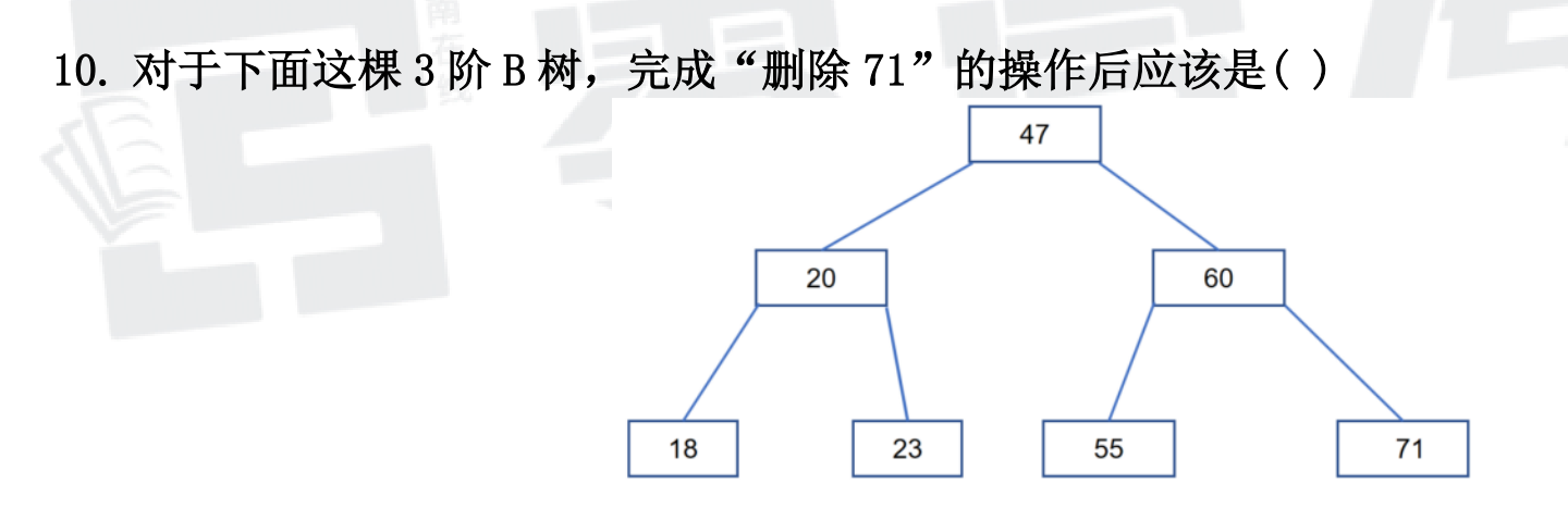
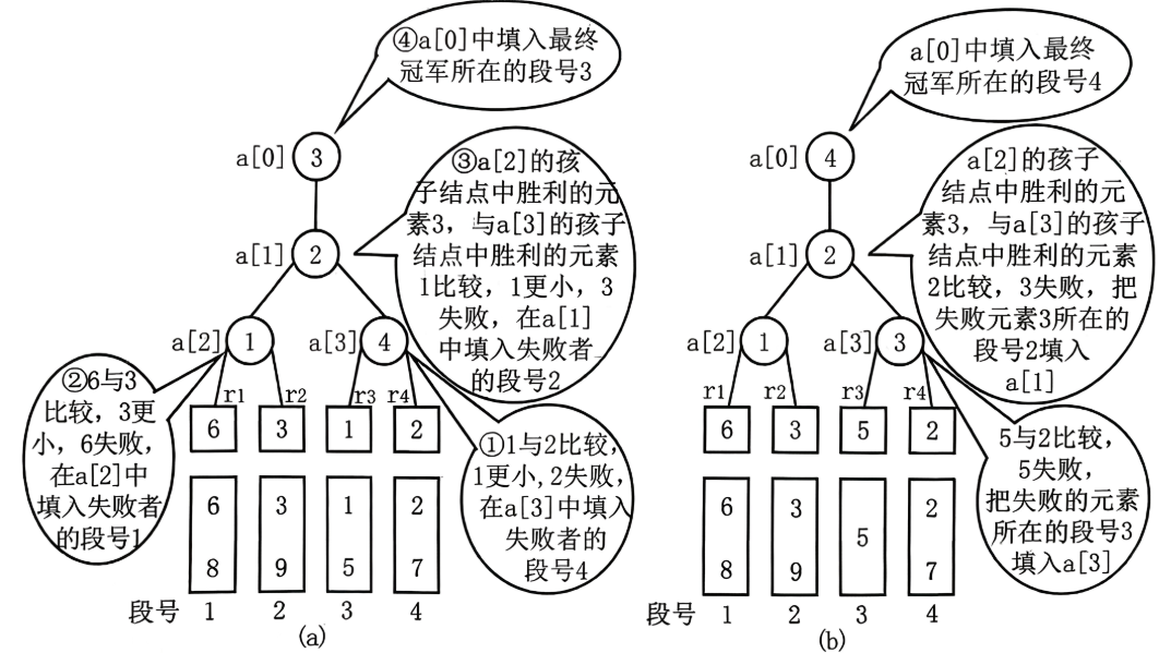
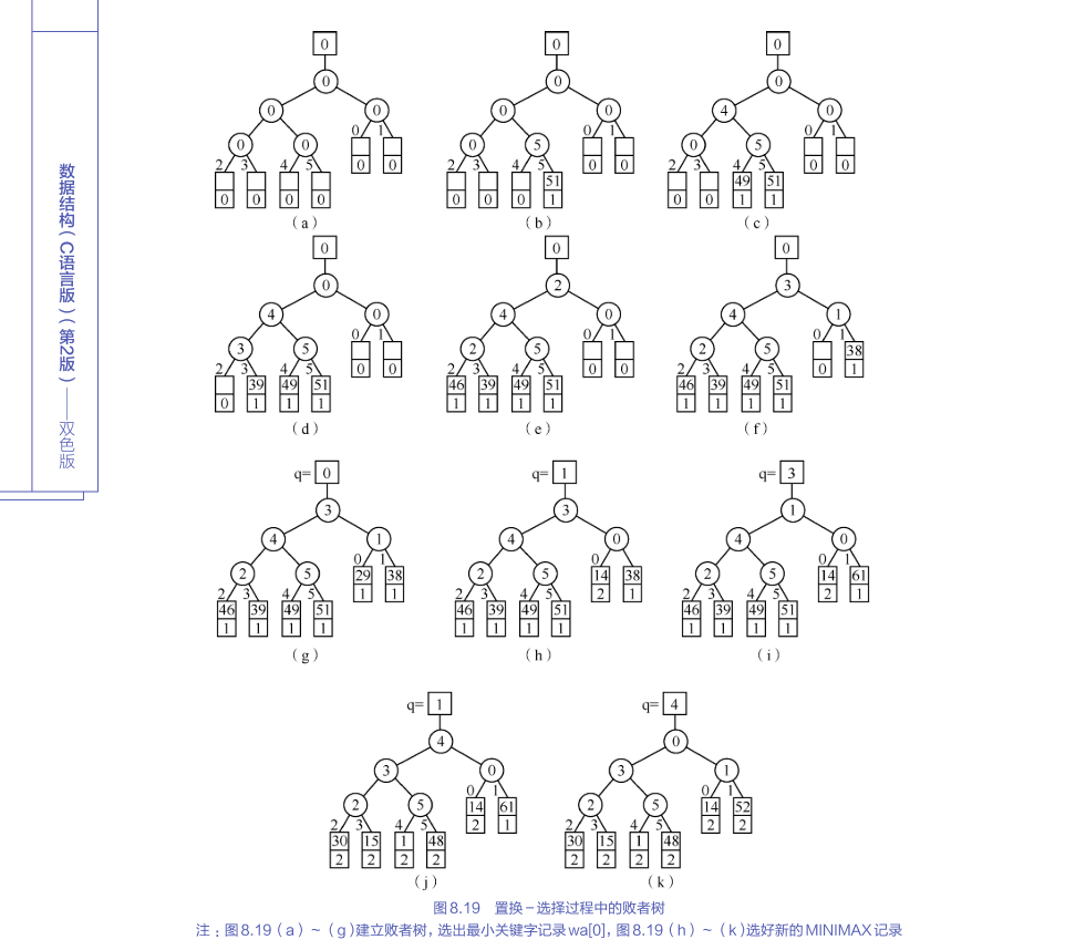
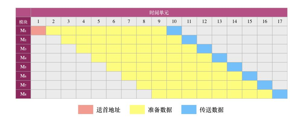
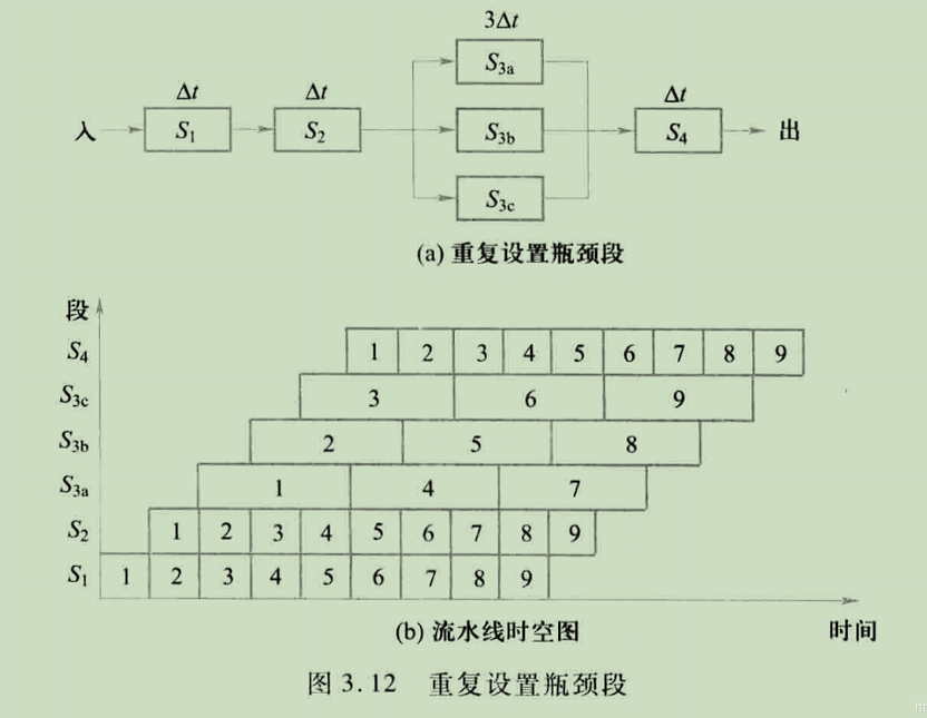
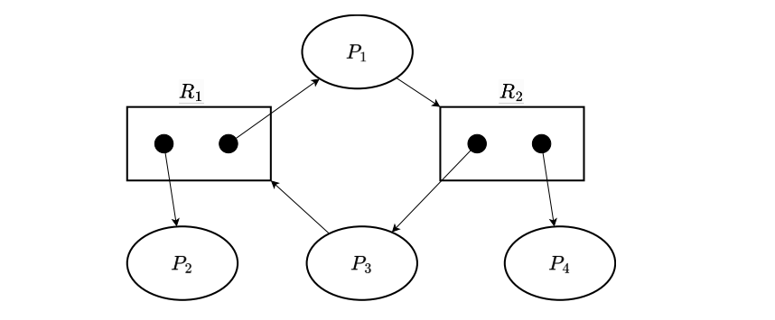
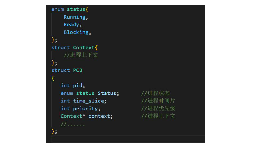
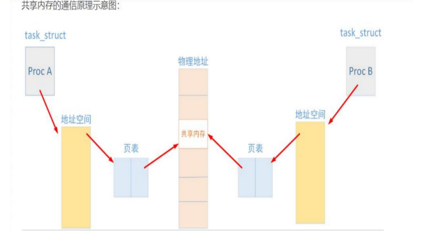
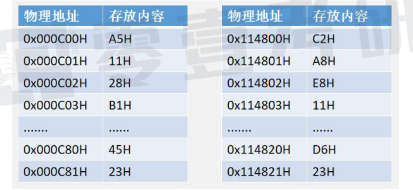
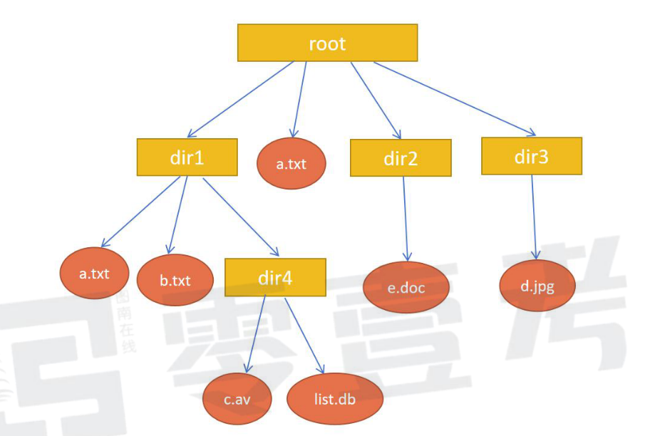
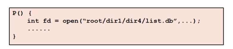
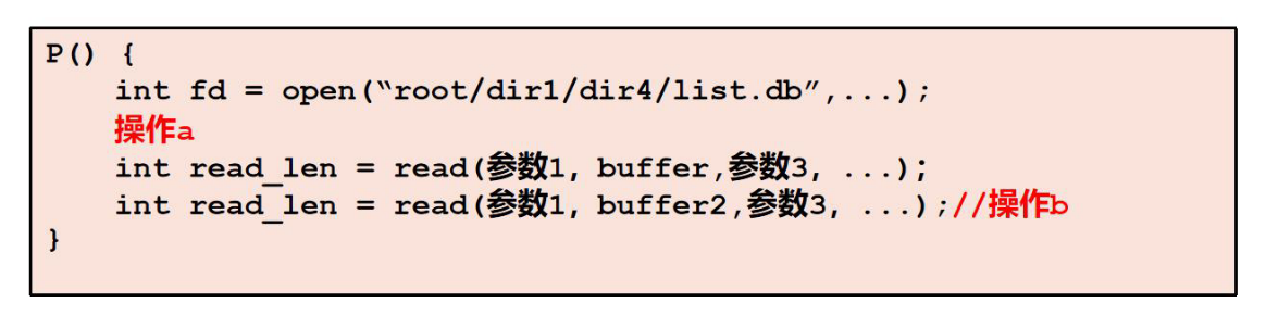
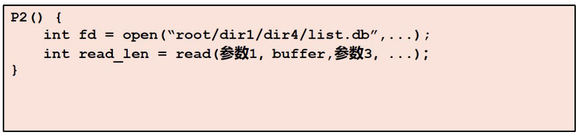
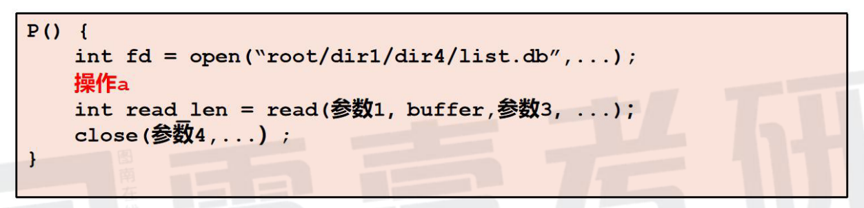
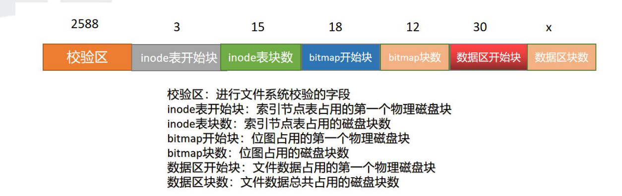
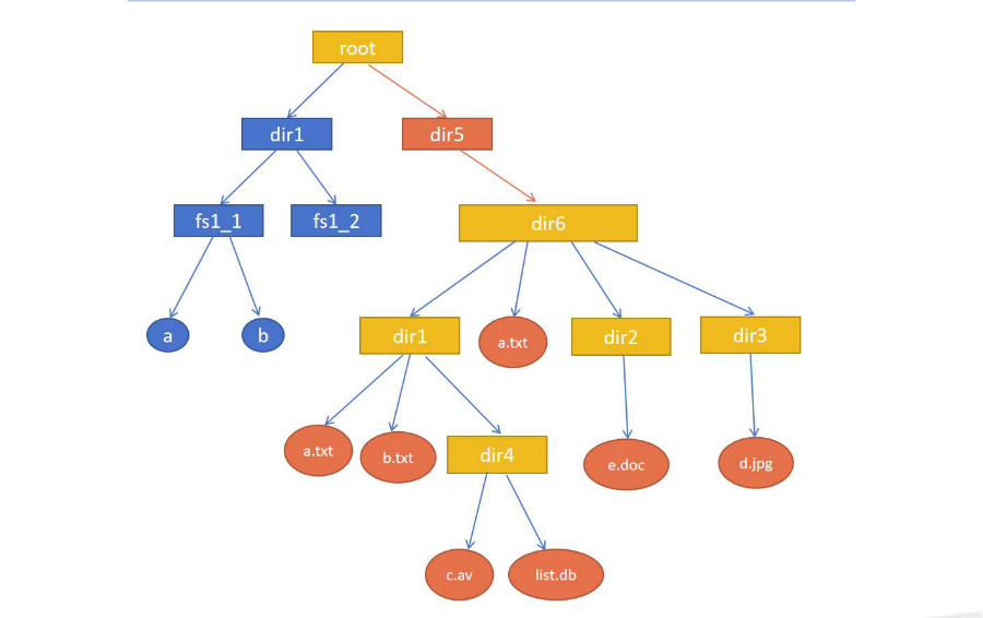
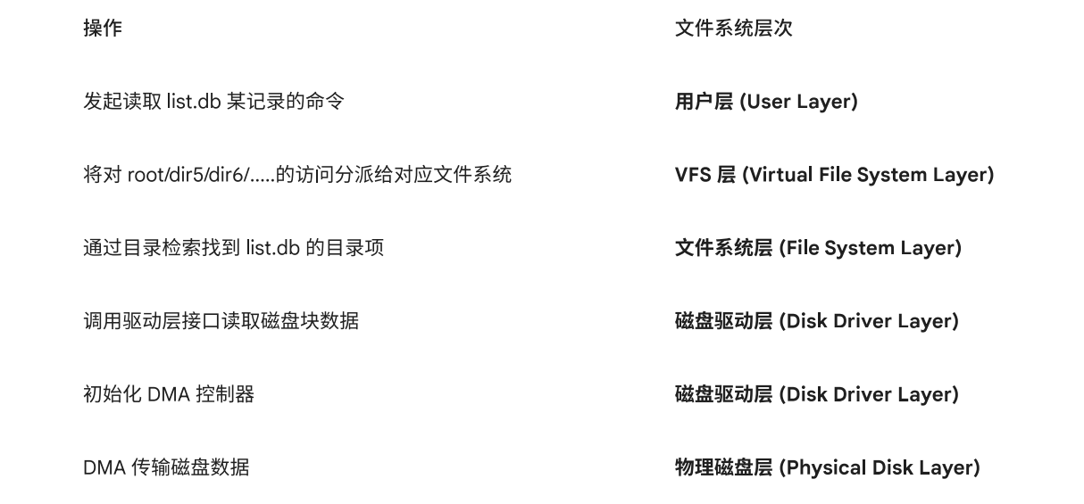
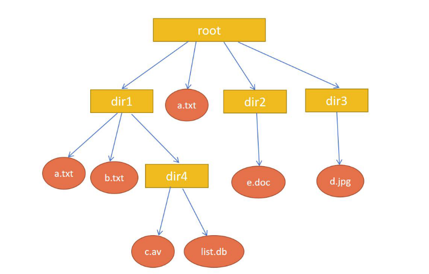
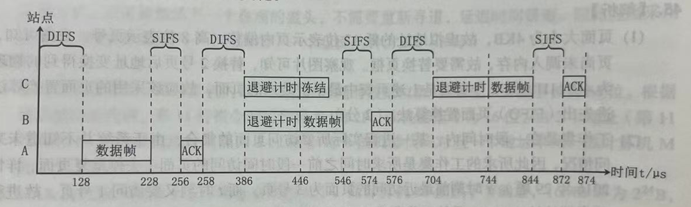
Comments