Algorithm Notes: The Grand Collection
Two years of algorithm study notes from my cnblogs blog, reorganized into seven chapters: basic algorithms, search, dynamic programming, data structures, strings, graphs, and math
This collection reorganizes the algorithm notes I wrote on cnblogs between 2023 and 2024 into seven chapters. The original reasoning, derivations, and code are preserved (including the asides I scribbled back then); places that only had code now carry explanations, and places that ran long were trimmed slightly. For the unabridged originals, follow the source-note links at the top of each section.
Chapter 1: Basic Algorithms
1.1 Prefix Sums and Difference Arrays
Prefix sums answer “sum of any interval, many queries”: after preprocessing $s_i = s_{i-1} + a_i$, the sum over $[l, r]$ is $s_r - s_{l-1}$. The 2D version unfolds by inclusion-exclusion: $s_{i,j} = s_{i-1,j} + s_{i,j-1} + a_{i,j} - s_{i-1,j-1}$.
///s[i][j] = s[i-1][j] + s[i][j-1] + a[i][j] - s[i-1][j-1]
printf("%d\n", s[x2][y2] - s[x2][y1-1] - s[x1-1][y2] + s[x1-1][y1-1]);
A difference array is the inverse: if $a$ is the prefix sum of $b$, “add $c$ on $[l,r]$” is just $b_l \mathrel{+}= c,\ b_{r+1} \mathrel{-}= c$, then one prefix-sum pass rebuilds the array.
Three problems tie it together in my second note: Laser Bomb (2D prefix sums over every frame — a 3×3 frame actually traps a 2×2 bomb, so start accumulating at (1,1)); Increasing Sequence (after differencing, with positive sum $res$ and negative sum $ans$, the answer is $\min(res,ans) + |res-ans|$ and the count of schemes is $|res-ans|+1$); and Classroom Reservations (difference array + binary search on the answer — check(mid) tests whether the first mid orders overflow, turning $O(nm)$ into $O((n+m)\log m)$; that note keeps my 45-point brute force beside the full version).
Source notes: 基础算法大全 · 再谈 前缀和,差分,离散化
1.2 Two Pointers and Coordinate Compression
The classic two-pointer problem: longest substring without repeats. The right pointer advances; on a duplicate the left pointer moves until the window is clean. Both pointers travel at most $n$ steps — amortized $O(n)$:
for (int i = 0; i < n; i++) {
    s[a[i]]++;
    while (s[a[i]] > 1) s[a[j++]]--;  // until the window has no duplicate
    res = max(res, i - j + 1);
}
Coordinate compression handles “huge value range, few distinct values”: sort and dedupe the coordinates that appear, binary search for ranks. Classic application — Program Analysis (P1955): indices reach $10^9$, so compression is mandatory. Merge all equality constraints first, then check each inequality constraint against the merged sets.
Source note: 基础算法大全
1.3 Fast Power and Big-Integer Arithmetic
Fast power turns $O(k)$ exponentiation into $O(\log k)$ by splitting the exponent into binary:
long long qpow(long long a, long long b, long long k) {
    long long res = 1;
    while (b) {
        if (b & 1) res = res * a % k;
        b >>= 1, a = a * a % k;
    }
    return res;
}
Big integers live in digit arrays (index 1 = ones place). Multiplication’s key fact: the product of position $i$ and position $j$ lands in position $i+j-1$:
c[i + j - 1] = a[i] * b[j] + t + c[i + j - 1];
t = c[i + j - 1] / 10;
c[i + j - 1] %= 10;1.4 Greedy
My greedy note was a sweep of interval models, one problem each:
- Interval point-cover / maximum disjoint intervals: sort by right endpoint, take greedily — “the earlier an interval ends, the more room it leaves” covers both questions.
- Minimum interval grouping: sort by left endpoint; a min-heap tracks each group’s maximum right endpoint. A new interval joins the group with the smallest right endpoint when they don’t intersect, otherwise it opens a new group. The heap size is the answer.
- Merging fruits: always merge the two smallest piles — a bare min-heap problem.
- Model transformations: radar placement maps each point to $[x-d, x+d]$ on the axis ($d=\sqrt{r^2-y^2}$), reducing to point-covering; Tian Ji’s horse racing uses best-vs-best, worst-vs-worst, and sacrifices the worst horse against their best; the fishing problem enumerates the final lake and repeatedly takes the highest-yield lake from a heap.
priority_queue<int, vector<int>, greater<int>> heap;
for (int i = 0; i < n; i++) {
    if (heap.empty() || heap.top() >= range[i].l) heap.push(range[i].r);
    else { heap.pop(); heap.push(range[i].r); }
}
printf("%d\n", heap.size());
Source note: 贪心算法
1.5 Regret Greedy
My most complete theoretical note, with the mountain-climbing metaphor: plain greedy always takes the currently best step and never looks back — which can trap you on a local peak. Regret greedy keeps an escape hatch: when a better choice appears, undo an earlier decision and climb the higher mountain.
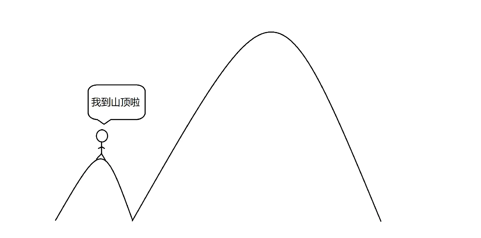
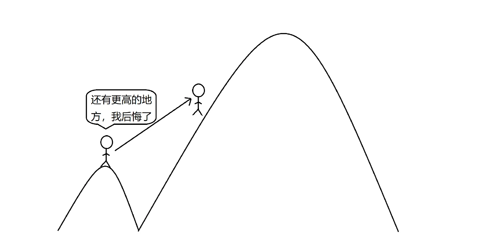
Two families by implementation: the regret heap (a heap tracks the worst-value decision made so far; a better new decision swaps it out) and the regret automaton (a difference decomposition that makes any greedy path converge to the global optimum).
Fixed-time model (Work Scheduling): sort tasks by deadline; if there’s time, do it and push its profit into a min-heap, otherwise swap out the lowest profit:
sort(v.begin(), v.end());
int now = 0, res = 0;
for (auto [x, y] : v) {              // x = deadline, y = profit
    if (x > now) res += y, now++, que.push(y);
    else if (!que.empty() && y > que.top())
        res += (y - que.top()), que.pop(), que.push(y);   // regret: drop lowest profit
}
Fixed-value model (Building Repair): equal values mean you swap out the longest task instead — a max-heap, mirrored logic.
Heap regret automaton (CF865D) rests on the identity
$$C_{sell} - C_{buy} = (C_{sell} - C_i) + (C_i - C_{buy})$$Push each day’s price once for the plain greedy; if today’s price beats the heap top, add the difference to the answer and push today’s price again as the intermediate variable $C_i$. When a real sale happens later, the differences cancel the middle term.
Doubly linked list regret automaton (Tree Planting): after choosing $B$ its neighbors $A, C$ die — but if the global optimum is $A+C$? Insert a node $P$ valued $a + c - b$; picking $P$ later equals regretting “$B$ out, $A+C$ in”. With a max-heap this is $O(n \log n)$. The four pitfalls from my note: skip deleted nodes; handle the 1-adjacent-to-n wraparound; don’t botch the linked list; write a new node’s value back to the array before pushing it into the heap.
Source note: 反悔贪心学习笔记
1.6 Binary Lifting
Any $k$ decomposes into powers of two, so precompute $f_{i,j}$ = position after $2^j$ steps from $i$ and answer queries by jumping high bits first, $O(\log k)$:
for (int j = 1; j < 20; j++)
    for (int i = 1; i <= 2 * n; i++)
        f[i][j] = f[f[i][j - 1]][j - 1];   // jump 2^j steps from i
Two representatives: Running (P1613, each second covers $2^k$ km — a Floyd-style triple loop computes $edge_{i,j,k}$ = “a path of length exactly $2^k$ from $i$ to $j$”, then connect all one-second-reachable pairs and run Dijkstra); National Flag Plan (P4155, circular interval covering — break the circle by duplicating the chain, lift to the covering endpoint; counting uses < rather than ≤ because the last step may land exactly on target, so undercount uniformly and add 1).
Source note: 倍增
Chapter 2: Search
2.1 DFS: The Two Basic Shapes
Permutation-style — n-queens: place row by row, mark columns and both diagonals ($u+i$ and $n-u+i$, the $+n$ guarding against negatives), recurse, restore:
if (!cow[i] && !dg[u+i] && !rdg[n-u+i]) {
    Q[u][i] = 'Q';
    cow[i] = dg[u+i] = rdg[n-u+i] = true;
    dfs(u + 1);
    cow[i] = dg[u+i] = rdg[n-u+i] = false;  // restore
    Q[u][i] = '.';
}
Binary-choice style — PERKET: every ingredient branches into add/don’t-add, enumerating subsets. Selecting Numbers (P1036) is the combination version: passing a start parameter so combinations never repeat.
2.2 BFS: Shortest Paths and Mark-on-Enqueue
BFS expands layer by layer; the first arrival is the shortest distance — maze shortest path and knight traversal are bare BFS. My knight note dissects an MLE+TLE: mark visited at enqueue time, not dequeue time — otherwise the same cell is queued once per neighbor and the queue explodes:
if (vis[x1][y1] == -1) {
    node next = {x1, y1, now.step + 1};
    vis[x1][y1] = now.step + 1;   // mark immediately
    que.push(next);
}
Extra constraints simply widen the state: meteor shelter (per-cell danger time; a pit can be struck twice, so keep the minimum), Naruto and Sasuke (chakra is part of the state — vis[x][y][chakra] goes 3D), Saving Tang Monk (keys + priority queue + snakes costing 2 steps), Corn Maze (teleport first, then expand — otherwise an infinite loop), ROADS (cost as a state dimension, layered shortest path). Flood fill (counting connected pastures) shows the DFS that never backtracks.
2.3 Memoized Search
Skiing: slide downhill, maximize path length. A cache array $f_{x,y}$ turns exponential re-computation into $O(nm)$. In my own words from that era: “every memoized search can be turned into DP, but not every DP can be turned into memoized search.”
int dfs(int x, int y) {
    if (f[x][y]) return f[x][y];   // cached: return directly
    for (int i = 0; i < 4; i++) {
        int x1 = x + dx[i], y1 = y + dy[i];
        if (a[x][y] > a[x1][y1])
            f[x][y] = max(f[x][y], dfs(x1, y1) + 1);
    }
    return f[x][y];
}
Source note: 滑雪 OJ3651
2.4 The Four Pruning Techniques
Take Big Westward Strips (P1118): brute-force permutations explode. High-school algebra first — the weighted sum $res = \sum c_i a_i$ uses Pascal’s triangle row $n$ as coefficients:
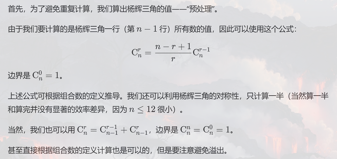
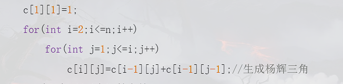
Then prune in four directions: optimize search order (try large values first); feasibility pruning (sum > k cuts immediately); optimality pruning; and excluding equivalent redundancy (vis[] per level, skipping equal-length rods in Sticks, recording failed lengths in fail, backtracking markers instead of memset).
bool dfs(int cnt, int num, int sum) {
    if (sum > k) return false;        // feasibility pruning
    if (cnt == n) { if (sum == k) { res[cnt] = num; return true; } return false; }
    vis[num] = true;
    for (int i = 1; i <= n; i++)
        if (!vis[i] && dfs(cnt + 1, i, sum + cow[cnt] * i)) { res[cnt] = num; return true; }
    vis[num] = false;                 // backtracking marker
    return false;
}
Source notes: 双端队列优化搜索,最优性剪枝,可行性剪枝,优化搜索顺序,排除等效冗余 · 搜索例题
2.5 Iterative Deepening and Bidirectional Search
Iterative deepening: set a depth cap; if no answer, raise it and retry. Re-searching looks wasteful, but tree size grows exponentially with depth, so the shallow layers are negligible. Bidirectional search (Gifts, $n \le 45$): split in half; preprocess all subset sums of the first half, sort and dedupe; for each subset sum of the second half, binary-search the first-half table for the largest sum within remaining capacity — $2^n$ drops to $2^{n/2} \cdot n$. Sorting descending first helps: “a larger current sum reaches the target faster, making the search shallower.”
Source note: 迭代加深,双向搜索,IDA*,A*,双端队列BFS
2.6 A* and IDA*
A* swaps BFS’s queue for a priority queue keyed by real distance + estimate; the estimate must not exceed the true remaining cost. The 8-puzzle uses Manhattan distance with string states in a hash map. IDA* = iterative deepening + estimate pruning: cut as soon as depth + f() > max_depth. Implementation notes from my own runs: tabulate the 8 rotations of the Rotation puzzle as index arrays; its estimate is 8 minus the most frequent color among the center 8 cells; exclude the move opposite to the previous one (they cancel). For knight color-swapping (P2324) the estimate is the larger of the two sides’ misplaced counts — one swap fixes at most one per side, a tight lower bound (that version ran in 300 ms).
int f() {   // UVA1343 estimate: 8 - max same-color count in the center
    int sum[4] = {0}, maxx = 0;
    for (int i = 0; i < 8; i++)
        sum[mp[center[i]]]++, maxx = max(maxx, sum[mp[center[i]]]);
    return 8 - maxx;
}
bool dfs(int depth, int max_depth, int lst) {
    if (depth + f() > max_depth) return false;   // IDA* pruning
    if (f() == 0) return true;
    ...
}Source note: 迭代加深,双向搜索,IDA*,A*,双端队列BFS
2.7 0-1 BFS with a Deque
For graphs whose edges are 0 or 1, Dijkstra is overkill: nodes reached by a 0-edge enter at the front of the deque, by a 1-edge at the back. Distances stay two-segmented and monotone; each node enters once; $O(nm)$. The circuit board problem (P4667) is the standard: grid points as nodes, the direction aligned with a cell’s diagonal costs 0, the perpendicular direction costs 1.
if (turn(a, b, x, y)) {                        // rotation needed, cost 1
    dis[x][y] = min(dis[x][y], dis[a][b] + 1);
    q.push_back({x, y});                       // back
} else {                                       // aligned, cost 0
    dis[x][y] = min(dis[x][y], dis[a][b]);
    q.push_front({x, y});                      // front
}
The same search-algorithms note also holds my full set of shortest-path templates (plain/heap Dijkstra, Bellman-Ford, SPFA with negative-cycle detection, Floyd, shortest-path counting) — see Chapter 6, section 6.1.
Source notes: 迭代加深,双向搜索,IDA*,A*,双端队列BFS · 搜索算法
Chapter 3: Dynamic Programming
3.1 The Knapsack Family
My introductory DP note opens with the method — “first write down the dynamic set, then compute dynamically” — and an indexing trick: “when the recurrence uses i−1, start i at 1 and you never go out of bounds.”
0-1 knapsack: the 1D optimization must iterate capacity downward:
for (int i = 1; i <= n; i++)
    for (int j = m; j >= w[i]; j--)   // descending: each item used at most once
        dp[j] = max(dp[j], dp[j - w[i]] + v[i]);
Complete knapsack differs by exactly one line — ascending capacity (“look closely: 0-1 and complete knapsack are extremely similar; figure out where the one-line difference comes from!!!!”). Bounded knapsack: brute force caps the k-loop at $s_i$; the real fix is binary splitting (“for s=200 the k-loop reaches 64, representing 1–127; the remainder takes one more item”), then run 0-1. Grouped knapsack adds an item-in-group loop. Dependent knapsack (Budget Plan, P1064): with at most 2 accessories per main item, enumerate the four cases — main only, main+acc1, main+acc2, main+both.
Source note: 动态规划dp
3.2 Linear DP: From Number Triangle to LCS
- Number triangle: $f_{i,j} = \max(f_{i-1,j-1}, f_{i-1,j}) + a_{i,j}$; initialize from the source or the borders become $-\infty$.
- LIS: $O(n^2)$ with $f_i = \max_{a_j
- LCS: the classic 2D board. The upgrade (P1439): renumber the first sequence to $1..n$, map the second through it, and LCS becomes LIS — $O(n \log n)$. “Ascending in the renumbered array = preserving the original order.”
- Edit distance (P2758):
min({dp[i-1][j]+1, dp[i][j-1]+1, dp[i-1][j-1]+(a[i]==b[j]?0:1)}).- Arithmetic-progression counting (P4933): $f_{i,d}$ = number of progressions ending at i with difference d; shift d by 20000 to stay non-negative.
3.3 Interval DP
Two loop templates, both from my notes. By length (Stones merging):
for (int len = 2; len <= n; len++)
    for (int i = 1; i + len - 1 <= n; i++) {
        int l = i, r = i + len - 1;
        dp[l][r] = 1e9;
        for (int k = l; k < r; k++)
            dp[l][r] = min(dp[l][r], dp[l][k] + dp[k+1][r] + s[r] - s[l-1]);
    }
By endpoints — “similar to Floyd in graph theory”, with the warning “the left endpoint must iterate in reverse, otherwise the traversal is incomplete”:
for (int i = n; i >= 1; i--)
    for (int j = i + 1; j <= n; j++) {
        dp[i][j] = 1e9;
        for (int k = i; k < j; k++)
            dp[i][j] = min(dp[i][j], dp[i][k] + dp[k+1][j] + s[j] - s[i-1]);
    }
The circular version (P1880) doubles the array (“cut the ring open and append a copy”), then take the best over all length-n windows. Treats for the Cows shows the power of defining $dp_{i,j}$ as “the interval $[i,j]$ not yet sold” — walking from the full interval down to single points, multiplying by the day of sale.
3.4 Tree DP and State-Machine DP
Tree knapsack (Course Selection, CTSC1997): a forest becomes a tree by adding a virtual node 0 — “node 0 must be chosen but has value 0”, the answer is f[0][m+1]. The transition is grouped knapsack over children, then squeeze u itself in with f[u][i] = f[u][i-1] + v[u].
State-machine DP: the stock series. Two transactions: $dp_{i,j,0/1}$ = day i, j completed trades, holding nothing/holding:
dp[i][j][0] = max(dp[i-1][j][0], dp[i-1][j][1] + w[i]);
dp[i][j][1] = max(dp[i-1][j][1], dp[i-1][j-1][0] - w[i]);
Pitfall from my note: “check all three cases — buying once may be optimal if a second trade would lose money; buying and selling immediately counts as the first trade’s maximum.” The cooldown variant splits states into holding / just-sold (frozen) / free — the transitions form a ring. Another flavor runs a KMP automaton inside DP (passwords avoiding a substring T): the second dp dimension is the match position in T, and each of the 26 letters advances it along the failure links; reaching position m is forbidden.
3.5 Bitmask DP
From my note: “state compression packs multiple flags into one integer — with m flags there are $2^m$ states; 0010 means only the second flag holds; merge states with |.” Three steps: Candy (preprocess each pack’s flavor set; $f_{j|candy_i} = \min(f_{j|candy_i}, f_j+1)$, $O(n \cdot 2^m)$); Mutual Exclusion (P1896 — first filter row-valid masks, then precompute pairwise compatibility !(a&b) && check(a|b), dp over rows × masks × king count); Eating Cheese (TSP shape, $f_{i,k}$ over visited-set k).
3.6 Monotone-Queue Optimized DP
The template intuition: “a monotone queue keeps its elements ordered; the answer (optimum) sits at the front, the newest element at the back. It maintains range extrema or removes a DP dimension.” Sliding window (P1886):
while (hh <= tt && q[hh] < i - k + 1) hh++;      // front out of window
while (hh <= tt && a[q[tt]] >= a[i]) tt--;       // back elements beaten by a[i] are useless
q[++tt] = i;
if (i >= k) cout << a[q[hh]] << ' ';
DP optimization (P1725): $f_i$ transfers from $[i-r, i-l]$ — the window slides as i advances, and “the newly entering element is $i-l$”. Hopscotch (P3957) = binary search on the answer + monotone queue: more gold means more freedom, so feasibility is monotone in g; inside check the window is $[d-g, d+g]$.
The bounded-knapsack optimization is the centerpiece of that note, derivation preserved: from $F[i][j] = \max\{F[i-1][j - k v_i] + k w_i\}$, write $j = a d + b$ (with $d = v_i$) and group by remainder b; within a group the candidates form a sliding-window maximum:
$$F[i][j] = \max\{F[i-1][b + k d] - k w_i\} + a w_i$$The auxiliary queue rule: “when M enters the primary queue, pop from queue B everything smaller than M and push M; when M leaves, if B’s front equals M, pop it too” — that is exactly the mysterious “monotone queue” of the Nine Lectures on Knapsack.
Source note: 单调队列及单调队列优化DP
3.7 Digit DP
The guiding principle: “compute high digits using results already computed for low digits.” Two schools in my note:
Recurrence (Digit Count, ZJOI2010): preprocess $dp_i$ = occurrences of each digit among i-digit numbers, via $dp_i = dp_{i-1}\cdot 10 + 10^{i-1}$ or $dp_i = i \cdot 10^i / 10$. To count over $[0, 324]$: common segments reuse $dp_{i-1}$; the top digit $0 \sim num_i{-}1$ each contribute $10^{i-1}$; finally remove the illegal leading-zero block ($cnt_0 -= 10^{i-1}$).
Memoized search: states $dp_{pos, sum, lead, limit}$. Windy numbers:
int dfs(int pos, int last, int lead, int limit) {
    if (pos == 0) return 1;
    if (last >= 0 && dp[pos][last][lead][limit] != -1) return dp[pos][last][lead][limit];
    int ans = 0, to = limit ? num[pos] : 9;
    for (int i = 0; i <= to; i++) {
        if (abs(i - last) >= 2)          // windy condition
            ans += dfs(pos - 1, i, false, limit && i == to);
    }
    dp[pos][last][lead][limit] = ans;
    return ans;
}lead tracks leading zeros; limit tracks whether we’re pinned to the upper bound — only limit && i == to keeps the pin. Digit-Sum-Divisible (P4127) pushes both the digit sum and its residue into the state: $dp[i][j][k][l]$, one run per candidate modulus (at most a 9·9 digit sum).
Source note: 数位 DP
3.8 Rerooting DP
Problem: for every root, the sum of depths. Brute force is $O(n^2)$; rerooting is $O(n)$:
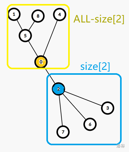
Root at 1, compute $dp_1$ and subtree weight sums $size_u$; then push from parent to child — the outside (yellow) gains $(ALL - size_x)\cdot w$, the inside (red) loses $size_x \cdot w$:
int ndp = cur;
ndp += (sum - sz[x]) * y - sz[x] * y;   // dp[x] = dp[u] + outside - inside
dfs2(x, u, ndp);
The note closes with a list of seven same-shape problems (“just change the edge weights or node weights”) plus an alternative: find the centroid (largest subtree ≤ half), then one dfs accumulates $c_x \cdot depth$.
Source note: 树上深度和问题 - 换根DP
Chapter 4: Data Structures
4.1 Union-Find
find with path compression is the soul (“hard to grasp at first — draw a picture”):
int find(int x) {
    if (p[x] != x) p[x] = find(p[x]);   // climb to the root
    return p[x];
}
Weighted union-find: Food Chain (P2024) stores d[x] = distance to parent, which path compression turns into distance-to-root (“save p[x] before recursing”); same species ⇔ (d[a]-d[b]) % 3 == 0, a eats b ⇔ %3 == 1. Same family: A Bugs (odd/even distances), Imprisoning Criminals P1525 (“the enemy of my enemy is my friend” — sort conflicts descending, remember each point’s first enemy in vis[x], merge enemy batches on the second sighting; the first conflict edge whose endpoints are already joined is the answer), Galaxy Heroes (depth-weighted: dep[u]=sz[v] on merge, answer abs(dep[a]-dep[b])-1), P1621 (union multiples of each prime ≥ k, count roots).
Source note: 并查集
4.2 Monotone Queue
Keeps the queue ordered with the answer at the front. Sliding window (P1886) — front evicted when out of window, back popped when beaten:
if (hh <= tt && i - k + 1 > q[hh]) hh++;      // front out of window
while (hh <= tt && a[q[tt]] >= a[i]) tt--;    // back beaten by the newcomer
q[++tt] = i;
if (i >= k - 1) cout << a[q[hh]] << " ";
Variants (P1440, P1638, 2D submatrix extrema “sweep rows first, then columns”) are rearrangements of these two steps.
Source note: 结构
4.3 Sparse Table for Static Range Extrema
The preprocessing explanation, preserved: “$f[i][j]$ is the maximum over the $2^j$ elements starting at i; merge two small intervals:
$$f[i][j] = \max(f[i][j-1],\ f[i+2^{j-1}][j-1])$$Like interval DP, iterate j (the length) before i. When j is fixed, i is confined to $[1, n-2^j+1]$; and $2^j \le n \Leftrightarrow j \le \lfloor\log_2 n\rfloor$.”
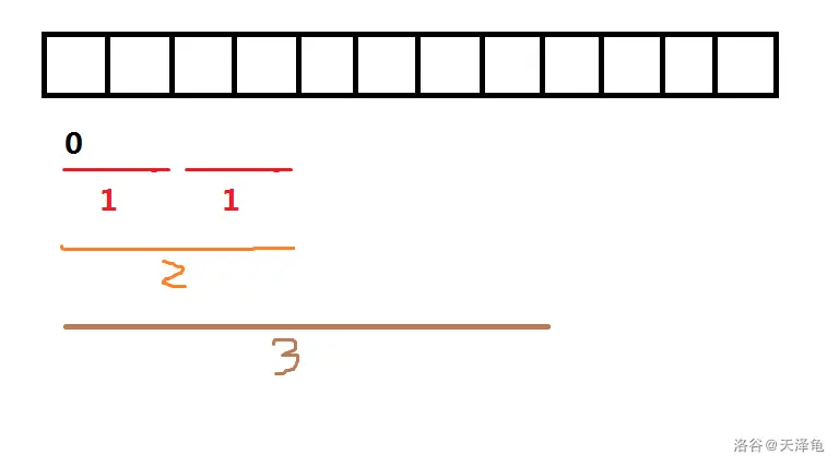
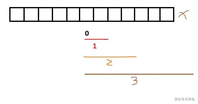
Queries glue two (possibly overlapping) blocks:
int pos = lg[y - x + 1];
cout << max(f[x][pos], f[y - (1 << pos) + 1][pos]) << endl;
Advanced: P7333 puts an ST table on a ring — triple the array (“i−mid can underflow during the binary search, so triple the space and binary-search from the middle”), each check reads $[i-x, i-1]$ and $[i+1, i+x]$.
Source note: 静态区间(一维和二维)最值问题
4.4 Fenwick Tree (BIT)
Its essence: “lowbit splits ranges into binary-aligned blocks… a Fenwick tree is a prefix sum that supports updates — faster, and maintains a wider variety of things.”
int lowbit(int x) { return x & -x; }
void add(int x, int c) { for (int i = x; i <= n; i += lowbit(i)) tr[i] += c; }
int sum(int x) { int op = 0; for (int i = x; i >= 1; i -= lowbit(i)) op += tr[i]; return op; }
Four applications of increasing trickiness: Loulan Totem (sweep twice for greater-on-left × greater-on-right and smaller×smaller); point query + range add (BIT over the difference array); range add + range sum (two BITs, $tr1$ on differences and $tr2$ on $i\cdot d_i$, prefix $= \sum tr1(x)(x{+}1) - \sum tr2(x)$); Mysterious Cow (assign ranks from the back — find the $(a_i{+}1)$-th remaining slot by binary-searching the k-th one in the BIT, then erase it).
Source note: 树状数组
4.5 Segment Tree
A supplement my original note promised but never wrote: a segment tree halves $[1,n]$ recursively; node u’s children are u<<1 and u<<1|1 in a 4N array. Point update and range query walk one root-to-leaf chain, $O(\log n)$; any range decomposes into at most $2\log n$ nodes. The universal skeleton is three functions: pushup (merge children into parent), build, modify/query.
Pseudo segment tree (point update, range query) — P1198, the minimal skeleton. Maximum subsegment sum upgrades “what to maintain”: each node stores range sum, max prefix, max suffix, and max subsegment, merged by w.all = max(l.all, r.all, l.rmax + r.lmax). Range GCD uses $\gcd(a,b,c)=\gcd(a, b-a, c-b)$: build over differences so range-add becomes two point-adds; answer $\gcd(\text{left sum}, \text{right gcd})$.
Lazy tags for range updates: “keep a mark on the parent only; push it down when a child is actually needed”:
void pushdown(int u) {
    auto &root = tr[u], &left = tr[u<<1], &right = tr[u<<1|1];
    left.sum += (left.r - left.l + 1) * root.lazy, left.lazy += root.lazy;
    right.sum += (right.r - right.l + 1) * root.lazy, right.lazy += root.lazy;
    root.lazy = 0;
}
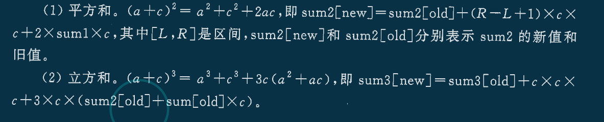
Multiply+add tags fix an operation order (multiply then add) inside one combined val() pushdown. Range XOR splits values into 21 bits, keeping should[i] = count of ones per bit; XOR-ing x toggles a per-bit reversal mark — after reversal the ones count is length minus the current count. Mixed tags (HDU4578: range add/multiply/assign, query sum of powers 1..3) uses three tags with two warnings from my note: “update in reverse order, like the knapsack — the previous change affects the next”, and pushdown order is fixed (assign → multiply → add):
Segment tree beats ($a_i = \min(a_i, x)$ over a range): maintain per node the max, second max, count of max, and sum. If $x \ge mx$, skip; if $se \le x < mx$, only maxes change — sum -= num * (mx - x); otherwise recurse. Amortized logarithmic. Practice: 最假女选手 (simultaneous min/max/add — full code in the original).
Persistent segment tree: a point update touches $\log n$ nodes, so clone only those and share the rest — “formally tr[new] = tr[old], then fix the left child; every version’s entry is its root”:
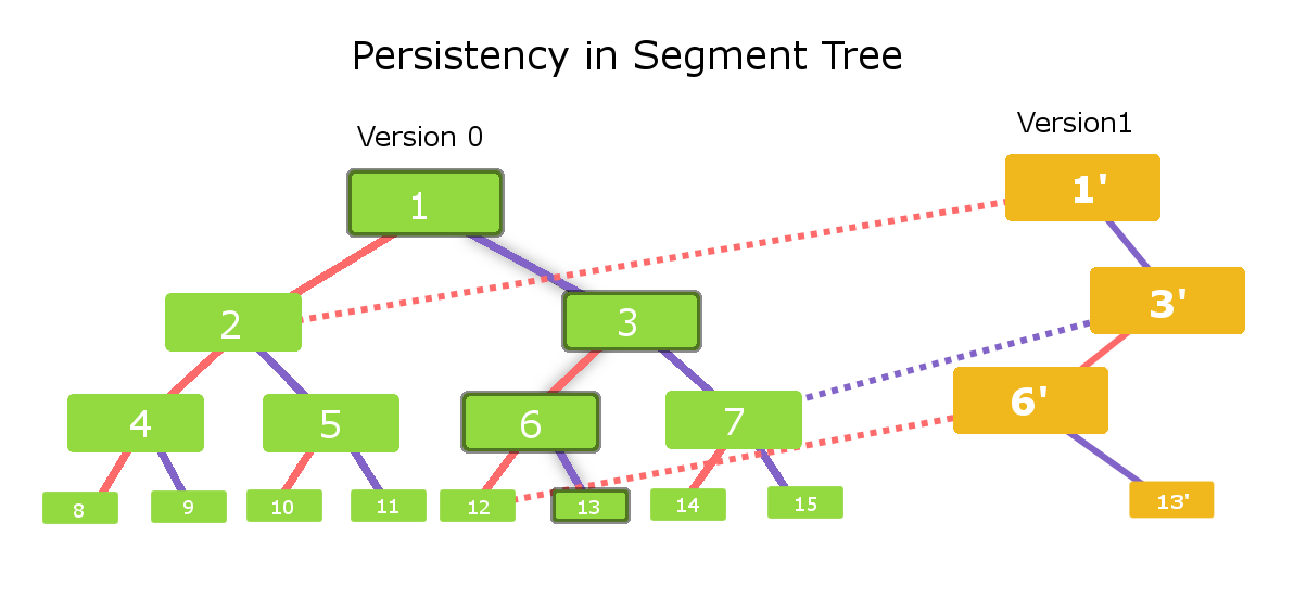
Template (persistent array) plus an application (ABC253F: range adds per version, row resets — query “current minus last-reset version” as a persistence difference).
4.6 Balanced Trees (FHQ Treap)
Why: “a BST given sorted data degenerates into a chain with O(n) operations; a balanced tree restores O(log n).” FHQ treap has only split (by value or by rank, into ≤v and >v) and merge (by heap order on random keys — “by normal distribution the tree height stays logarithmic”):
void split(int u, int v, int &x, int &y) {
    if (!u) return x = y = 0, void();
    if (tr[u].val > v) y = u, split(tr[u].l, v, x, tr[u].l);
    else x = u, split(tr[u].r, v, tr[u].r, y);
    pushup(u);
}
int merge(int x, int y) {
    if (!x || !y) return x + y;
    if (tr[x].key > tr[y].key) { tr[x].r = merge(tr[x].r, y); pushup(x); return x; }
    else                       { tr[y].l = merge(x, tr[y].l); pushup(y); return y; }
}Erasure splits twice (“split ≤x and >x, then split again at x−1; the second tree’s root must equal x — merge its children back. However you split it, merge it back”). Insert / rank / k-th / predecessor / successor are all split+merge combinations; interval reversal splits by rank and flips a lazy tag. Applications: P4309 maintains LIS under insertions by rank-splitting (“the new node’s answer is the max dp in the tree before it, plus one — and splitting never severs the parent of the current node”); CF702F splits by value and brute-force rebuilds the $[v, 2v)$ stretch that loses monotonicity.
Source note: 平衡树
4.7 Sqrt Decomposition
When to use it: “when normal data structures fail (too many dimensions, or memory blows up), or when the solution needs 3+ logs. Watch the data range — block solutions are $O(\sqrt n)$ or worse.” How: “pick a block size B; incomplete blocks at the ends are handled by brute force; for a query range, brute-force the two end blocks and put a tag on whole blocks.” The Magician (P2801) keeps a sorted copy e[] per block: updates brute-force the ends + tag whole blocks; queries count ≥c by brute force + lower_bound per whole block. Another problem exploits a decreasing-contribution bound — each update affects at most ~6 positions, so “the block size must be at least 6; 10 to be safe.”
Source note: 分块–解决区间问题
4.8 Mo’s Algorithm
My opening line: “an algorithm I thought I’d never meet — turned out to be elegant brute force. Brilliant.”
Sort queries with the left endpoint by block and the right endpoint within blocks; move two pointers. Complexity, from my note: with $x_i$ left endpoints in block i, block i costs $O(x_i\sqrt n)$; crossing blocks costs $O(\sqrt n)$ up to n times — $O(n\sqrt n)$. Right endpoints are sorted within each of $\sqrt n$ blocks, at most n moves each — $O(n\sqrt n)$. Total with sorting: $O(n\sqrt n)$.
sort(q + 1, q + 1 + m, [](Query x, Query y) {
    return pos[x.l] == pos[y.l] ? x.r < y.r : pos[x.l] < pos[y.l];
});
int l = 1, r = 0;
for (int i = 1; i <= m; i++) {
    while (q[i].l < l) add(--l);
    while (q[i].r > r) add(++r);
    while (q[i].l > l) del(l++);
    while (q[i].r < r) del(r--);
    ans[q[i].k] = res;
}Three drills: Little B’s queries ($\sum cnt^2$ maintained incrementally as ans += 2*cnt-1), Repeated Numbers (double counting of counts), Compressed Transformation (distinct values since last occurrence). The comparator’s (pos[l]&1)?r<w.r:r>w.r is the parity optimization — odd blocks sort right endpoints ascending, even blocks descending, halving right-pointer travel.
Source note: 莫队
4.9 Binary Trees and an STL Cheat Sheet
The terminology note is a solid reference; the code covers four problem types: depth (P4913), rebuild from preorder+inorder and print postorder (P1827 — find the root in the inorder, split, recurse), the reverse (P1030 — root is the last of postorder), and P1229’s elegant conclusion: count positions where s[i]==ss[j] && s[i+1]==ss[j-1] — nodes with exactly one child — the tree shape count is $2^n$ (“if preorder has AB, two possibilities; if postorder has BA, the sibling case is excluded — B must be A’s only child”). P3884 adds BFS-based LCA with tree depth and width.
STL sheet: set dedupes and sorts; lower_bound/upper_bound return iterators (grab predecessors with --it; insert ±huge sentinels first). multiset allows duplicates — erase(x) removes all copies while erase(it) removes one; P5076 passes as a balanced tree with a plain multiset. The string note (find/substr/replace/insert/erase, npos = 4294967295) works as a manual.
Chapter 5: Strings
5.1 KMP and the next Array
Both index conventions, preserved (“they’re essentially the same, just shifted”):
for (int i = 2, j = 0; i <= m; i++) {          // build next
    while (j && s2[i] != s2[j + 1]) j = ne[j];
    if (s2[i] == s2[j + 1]) j++;
    ne[i] = j;
}
for (int i = 1, j = 0; i <= n; i++) {          // match
    while (j && s1[i] != s2[j + 1]) j = ne[j];
    if (s1[i] == s2[j + 1]) j++;
    if (j == m) cout << i - j + 1 << endl, j = ne[j];
}Two classic properties: shortest period (Radio Transmission, P4391) — “if the string is periodic, $n - ne[n]$ is the shortest period; next can never record how many times the first period repeats” — the answer is one line, cout << n - ne[n]; and minimum common prefix-suffix (POI2006 OKR-Periods of Words) — shrink next all the way to 0 per prefix, answer $\sum i - j$, with the memoization trick if (ne[i]) ne[i] = j; (“jump straight to the final j to cut the enumeration”).
Source notes: 字符串(KMP, Trie树, STL) · kmp的神奇之处 · POI2006 OKR-Periods of Words
5.2 The Magic of KMP
Two off-label uses. First: replace equality with order comparisons — to test whether a pattern sits element-wise ≤/≥ some window of an array, change the match condition (“same matching scheme, just a different comparison”), then binary-search the pattern length:
while (j && a[i] < good[j + 1]) j = ne[j];   // fail: follow next
if (a[i] >= good[j + 1]) j++;                // match: elementwise >=
if (j == 2 * u - 1) return true;
Second (an ABC problem): with $T = A + inv_B + inv_A + B$, the condition becomes $A + inv_B = inv_A + B$ — flip half the string and run KMP, walking the next chain to collect all “suffix-matches-prefix” cut points (for (int i = 2*n; i; i = ne[i-1]) if (i <= n) ok[i]++;); a cut point valid in both directions splits the string.
Source note: kmp的神奇之处
5.3 Trie
Static 26-way arrays; insert creates missing children, terminal counters answer existence queries:
void Insert(char str[]) {
    int p = 0;
    for (int i = 0; str[i]; i++) {
        int u = str[i] - 'a';
        if (!son[p][u]) son[p][u] = ++idx;   // create missing child
        p = son[p][u];
    }
    cnt[p]++;
}
Drills: Wrong Roll Call (Trie for existence + map for duplicates → OK/WRONG/REPEAT), Magic Password (longest prefix chain via LIS with s[i].find(s[j])==0), Longest Prefix (P1470 — two solutions: mark all KMP endpoints of every dictionary word then dp; or bucket a set by word length and try substr cuts).
Source note: 字符串(KMP, Trie树, STL)
Chapter 6: Graph Theory
6.1 Shortest Paths and Minimum Spanning Trees
My pinned graph-theory note is a template compendium. Heap Dijkstra ($O(m \log n)$), with my original comments:
priority_queue<pii, vector<pii>, greater<pii>> que;
que.push({0, s});  // must be {0,s}: the heap orders by the first field, distance
while (!que.empty()) {
    auto now = que.top(); que.pop();
    int dis = now.first, head = now.second;
    if (vis[head]) continue; vis[head] = true;  // otherwise complexity degrades
    for (int i = h[head]; ~i; i = ne[i]) {
        int j = e[i];
        if (dist[j] > dis + w[i]) { dist[j] = dis + w[i]; que.push({dist[j], j}); }
    }
}Tricks in the same note: many-to-one (P1629 — “just build the graph backwards”, run Dijkstra twice); shortest-path counting (BFS: dist[v] > dist[u]+1 resets cnt[v] = cnt[u], == accumulates — “distinguish > and ==, don’t only handle >”); Bellman-Ford (edge-count-limited, relax from a backup snapshot to avoid same-round contamination); SPFA negative-cycle detection (cnt[v] >= n means a negative cycle — “an edge count beyond n obviously means a negative cycle”; push all nodes initially if the start may not reach the cycle); Floyd ($O(n^3)$) plus three applications — transit planning, reachability transitivity (d[j][k] |= d[j][i] && d[i][k]), Cow Contest (i beats j iff g[i][j] < inf; both counters ≥ n−1 fixes a rank), and emergency reconstruction (add repaired stations to Floyd one by one in time order); layered graphs (k free flights: k copies of the graph, 0-weight edges between layers; connect all copies of the terminal with 0 — “you may not need all k free flights”); difference constraints — my full theory comment is preserved in the original: “$x_i \le x_j + c_k$ becomes an edge $x_j \to x_i$ of weight $c_k$; add a super source 0 reaching every node; run single-source shortest path. A negative cycle means no solution; otherwise dist is a feasible solution. For minimum values run longest paths; for maximum values run shortest paths.” Candy (P3275) converts the five relation types; note cnt >= n+1 when starting from 0, and “a stack-based SPFA is sometimes faster than the queue version.”
MST: plain Prim (“initialize all distances to infinity; each round take the nearest point and update”) and Kruskal (“sort edges by weight; add an edge when its ends are disconnected”). Applications with twists: buying gifts (gifting yourself = edges from node 0 of weight m, then MST), Pocket Sky (n nodes into k components = keep n−k edges, stop early), Rescue (“reverse thinking” — maximize deleted cost = add edges descending; never rebuild between two enemy nodes, and a normal node joined to an enemy becomes one — “otherwise you can detour through an intermediate node and isolation fails”).
6.2 LCA Three Ways
Binary lifting — my note’s steps: “fa[i,j] = the node 2^j steps up from i; sentinel: fa[i,j] = 0 when the jump overshoots the root, depth[0] = 0. Steps: [1] lift both nodes to the same depth; [2] jump both up until just below their LCA.”
int lca(int a, int b) {
    if (depth[a] < depth[b]) swap(a, b);
    for (int k = 15; k >= 0; k--)
        if (depth[fa[a][k]] >= depth[b]) a = fa[a][k];   // same depth first
    if (a == b) return a;
    for (int k = 15; k >= 0; k--)
        if (fa[a][k] != fa[b][k]) a = fa[a][k], b = fa[b][k];
    return fa[a][0];
}
Tarjan offline ($O(n+m)$): “during DFS, every node is in one of three states — [1] visited and backtracked, [2] on the current search path, [3] unvisited.” Answering (u,v) when v is in state [1]: the LCA is find(v), distance dist[u]+dist[v]-2*dist[anc]. HLD-based LCA: three lines (see 6.7).
Source note: 图论
6.3 Topological Sort
Peel leaves off a DAG. Base template plus three flavors: Bonus (top[j] = top[now]+1 pays layer by layer; the note also gives a difference-constraints alternative — super source, longest path); Station Grading (P1983 — stops point to every non-stop in their span; level = longest chain + 1; mp[][] guards against duplicate edges — “keep mp small or it MLEs”); Nastya and Potions (topological DP, min of buying directly — “mind the edge direction: ingredient points to product”).
queue<int> que;
for (int i = 1; i <= n; i++) if (p[i] == 0) que.push(i);
while (!que.empty()) {
    int now = que.front(); que.pop();
    for (int i = h[now]; ~i; i = ne[i])
        if (--p[e[i]] == 0) que.push(e[i]);
}
Source note: 图论
6.4 Tarjan, SCCs, and Undirected Connectivity
My theory comment, preserved: “dfn[u] is the timestamp when u is visited; low[u] is the smallest timestamp reachable from u. u is the highest point of its SCC iff dfn[u] == low[u].” When the bottom is reached, the whole stack segment pops as one SCC, and the numbering is a reverse topological order:
void tarjan(int u) {
    dfn[u] = low[u] = ++times;
    _stack[++top] = u, vis[u] = true;
    for (int i = h[u]; ~i; i = ne[i]) {
        int j = e[i];
        if (!dfn[j]) tarjan(j), low[u] = min(low[u], low[j]);
        else if (vis[j]) low[u] = min(low[u], dfn[j]);
    }
    if (dfn[u] == low[u]) {
        int y; ++scc_num;
        do { y = _stack[top--]; vis[y] = false, id[y] = scc_num; } while (y != u);
    }
}Applications: Popular Cows (after contraction, count out-degrees — the unique out-degree-0 SCC’s size is the answer; two or more → 0); contraction + longest path (“rebuild a fresh adjacency list and never reset the old one”; “it’s id[i], not id[j] — we compare each node with its neighbors”; SCC weights go into a new array); maximum semi-connected subgraph (dedupe contracted edges via hash = x*M+y in an unordered_set; “after contraction the numbering is already a reverse topological order — just sweep backwards”, counting schemes in parallel).
Bridges and edge-biconnectivity (P2860): paired edge encoding — i^1 is the reverse edge, the parent-edge check is i != (from^1); dfn[u] < low[j] marks a bridge (“j cannot reach anything at or above u”). After contracting eDCCs, count leaves of degree 1: the answer is (res+1)/2 — “the number of bridges needed to make a graph edge-biconnected is res/2 rounded up.” Listing bridges (P1656) is the same with output.
Source note: 图论
6.5 Centroid of a Tree
The definition from my note: “the centroid is the node whose largest subtree is as small as possible; deleting it leaves the most balanced forest.” One dfs computes subtree sizes, $f_u = \max(\max_{son} size_{son},\ n - size_u - 1)$, and the minimum f is the centroid (Meeting, P1395 — g[u] += g[j]+1 accumulates in-subtree distances; reroot at the centroid and sum).
Source note: 树的重心
6.6 Pseudo-Trees (基环树)
A systematic tutorial. The definition, verbatim: “strictly speaking, a pseudo-tree is not a tree — it is a graph with n nodes and n edges.” An undirected connected n+n graph is a tree plus one extra edge, hence exactly one cycle:
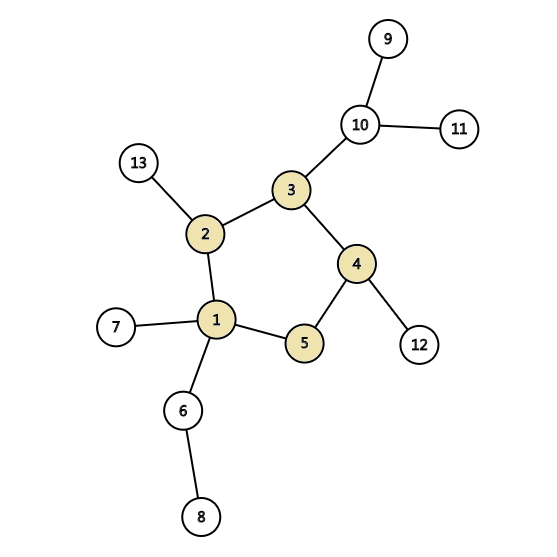
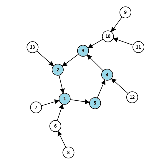
Directed versions: in-trees (each node has exactly one outgoing edge):
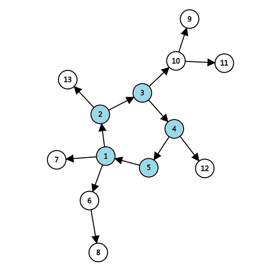
and out-trees (exactly one incoming edge):
The general recipe: “don’t panic — find the unique cycle; process everything outside the cycle as trees; then combine with the cycle.” Cycle-finding by DFS coloring, in my own words: “start anywhere; newly expanded nodes turn gray, backtracked nodes turn black; repeat until an untraversed edge expands into a gray node; paint that gray node red and return true; paint backtracked nodes orange; stop when the red node is reached.” The animation:
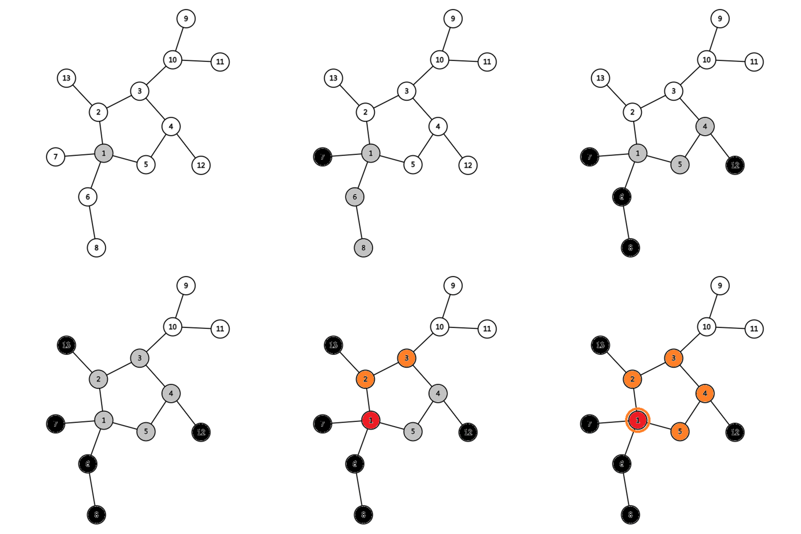
Forest marking tricks (pre-mark each component via another DFS; a second tag when processing cycle-less subtrees; or union-find at build time) plus the implementation detail: “expansion is legal only along untraversed edges — undirected edges are built in pairs, so mark both i and i^1.” What remains is “usually a tree DP on the subtrees, plus a linear DP with a monotone queue on the cycle (break the cycle into a chain and duplicate it).”
Two functional-graph applications from my 2024 revisit: Reachability in Functional Graph (an in-tree forest — each node’s answer is its distance to the cycle plus the cycle size; find cycles per component, memoize); Permute K times (same reduction becomes k-th ancestor — binary lifting $g(j+1,i) = g(j, g(j,i))$, $O(n \log k)$).
Source note: 基环树
6.7 Heavy-Light Decomposition
“Never studied it systematically before today — amazing that a tree structure supports this many operations.” Concepts (with my figure): heavy son (child with the largest subtree — exactly one), light sons, heavy edges, heavy chains, and chain heads (the shallowest node of a chain):
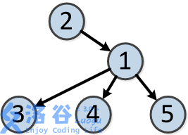
The complexity proof, preserved: “for a binary tree, a light edge’s subtree is at most half the size. Moving between heavy chains crosses a light edge, shrinking the subtree below 1/2 — so any node reaches the root across at most logn light edges (multi-way trees shrink even faster).”
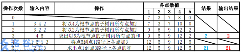
The LCA core is three lines:
int lca(int a, int b) {
    while (top[a] != top[b]) {                        // different chains: jump the deeper head
        if (dep[top[a]] > dep[top[b]]) a = fa[top[a]];
        else b = fa[top[b]];
    }
    return dep[a] > dep[b] ? b : a;                   // same chain: the shallower one
}
For the full template, the key observation is “within a heavy chain, dfs orders are consecutive — and so are they within a subtree”, so tree problems become segment tree problems:
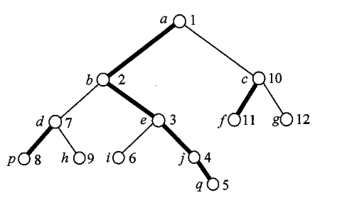
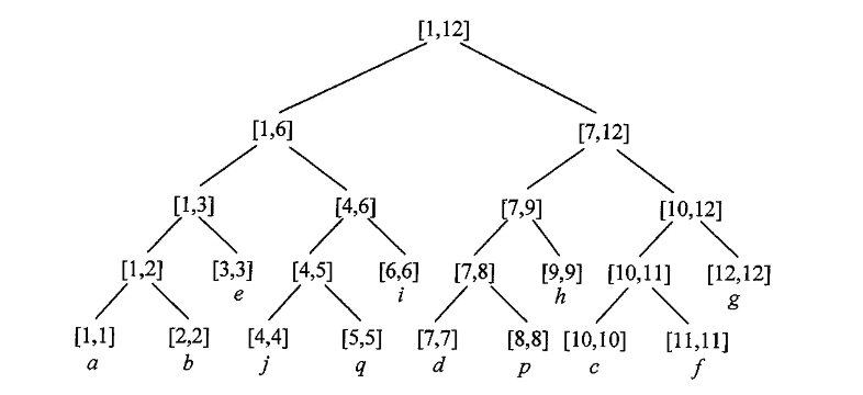
Path updates/queries hop chains exactly like the LCA (“modify the deeper chain’s range, jump the light edge, repeat until same-chain, then handle the small range”); subtree updates are one range call modify(1, id[x], id[x]+sz[x]-1, z). Total: $O(m\log^2 n)$. The complete implementation (segment tree + dfs1/dfs2 + update/get) is in the original.
Source note: 树链剖分
6.8 Centroid Decomposition
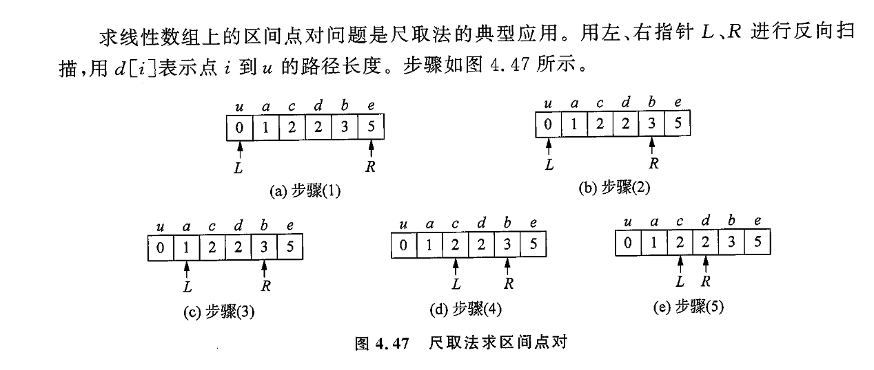
“Centroid decomposition is a divide-and-conquer over weighted-tree paths, taking brute force $O(n^2)$ down to $O(n \log n)$.” The template task: count pairs whose path length ≤ k (POJ1741). The split (from my note): “pick a node t; paths either pass through t or not. Paths avoiding t live in the subtrees left after deleting t — recurse.” Paths through t: one dfs collects all distances to t, sort, then two pointers:
Illegal paths sneak in: “with k = 7, if R reaches both X and Y at distance 3, the pair is counted — but the real route is R→X→R→Y, length 9; not a simple path. Any path whose two ends share a subtree is illegal.”
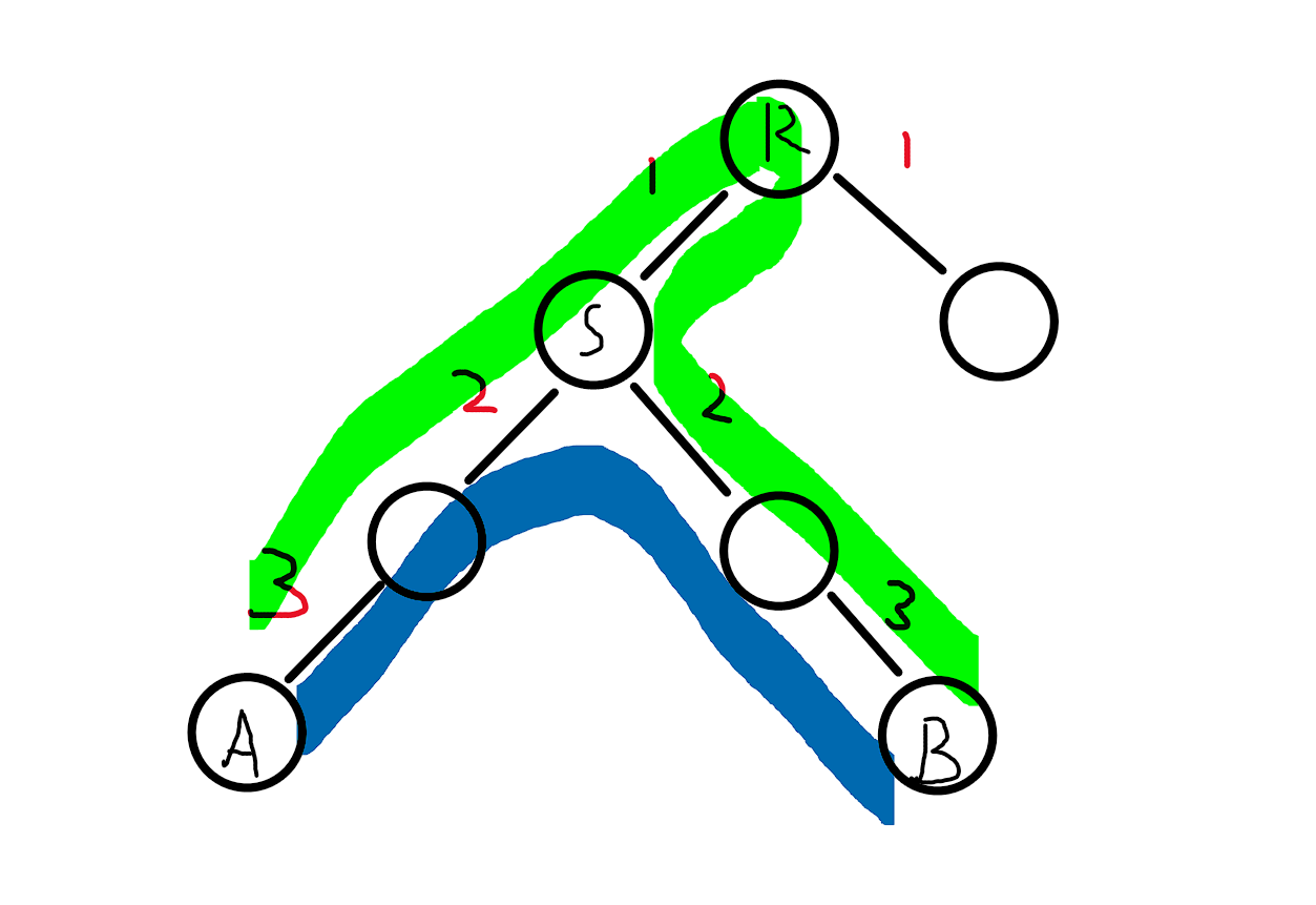
The fix: “count the subtree rooted at each child with k replaced by $k + w_{R \to S}$, and the illegal paths cancel out.” And the crucial part — the centroid: “always root at the centroid; every split leaves subtrees of size ≤ n/2, so recursion depth is only logn. Recursion logn × per-node nlogn = $O(n\log^2 n)$.”
void dfs(int u) {
    res += dfs3(u, 0);                 // count paths through u (with duplicates)
    vis[u] = true;
    for (auto [x, w] : g[u]) {
        if (!vis[x]) {
            res -= dfs3(x, w);         // remove same-subtree illegal paths
            now = 0, Tsize = sz[x], dfs1(x, 0);   // find the centroid
            dfs(now);                  // recurse
        }
    }
}Variants: P3806 (does a length-exactly-k path exist — “binary search is convenient, but don’t rerun the decomposition per query; the constant is large — just count directly”), ABC359G (same-color pair distance sums — maintain global sum[color] and cnt[color]; before entering child v add res += sum[A_v] + dist_v * cnt[A_v], then roll back per subtree).
Source note: 点分治详解(附图附例题)
6.9 Kruskal Reconstruction Trees, SPT, and Bipartite Covers
Kruskal reconstruction tree: “like a bottleneck tree — the (max or min) edge weight along the simple path between any two nodes equals their LCA’s value.” Build it while running Kruskal: each union creates a new internal node whose value is the merged edge’s weight, hanging the two roots beneath. Properties: heap-ordered from leaf to root; the bottleneck between two nodes is their LCA’s value. Typical use — “which nodes are reachable using only edges ≤ x”: find the shallowest ancestor with value ≤ x; its subtree is the answer. The original walks through the construction in eight figures.
Shortest path tree: run Dijkstra once from the source and keep only tree edges satisfying dist[v] == dist[u] + w; every node’s tree distance equals its graph distance, so “effect of deleting an edge” or “dp on trees” problems can run on the SPT.
Minimum vertex cover (bipartite, König): maximum matching = minimum vertex cover; Hungarian augmentation finds the matching, the cover is constructed from it.
DAG longest/shortest path: dp in topological order (dist[j] = max(dist[j], dist[i]+w) starting from in-degree 0), or contract SCCs first (see 6.4).
Source notes: Kruskal重构树 · 最短路径树SPT · 最小点覆盖问题 · DAG求最长路/最短路方法 · 最大食物链计数
Chapter 7: Math
7.1 Primes and Sieves
Trial division $O(\sqrt n)$ (i <= n/i to avoid overflow), Eratosthenes, then the Euler (linear) sieve — each composite is crossed out exactly once by its smallest prime factor:
for (int i = 2; i <= n; i++) {
    if (!vis[i]) prime[++res] = i;
    for (int j = 1; prime[j] <= n / i; j++) {
        vis[prime[j] * i] = true;
        if (!(i % prime[j])) break;   // prime[j] is i's smallest factor; further j would repeat
    }
}
The linear sieve carries extra payloads for free — P8795 records each number’s largest prime factor via p[i*prime[j]] = max(p[i], prime[j]): “always pick the largest prime factor, only then is the minimum as small as possible.” Factorization divides out primes up to $\sqrt n$; whatever remains (>1) is itself a prime factor.
Source note: (数论)素数,质数
7.2 Divisors and GCD
Trial division collects divisor pairs ($d \mid n \Rightarrow n/d \mid n$) into a set. The divisor-count formula comes from unique factorization: $\prod (k_i + 1)$. The sum of divisor counts over 1..n uses a sieve — my own explanation: “1 divides everything, 2 divides every multiple of 2 … a is b’s divisor iff b is a’s multiple: $1 + n/2 + n/3 + \dots = n \log n$.” GCD is one line — return b ? gcd(b, a%b) : a; (“gcd(a,b) equals gcd(b, a%b)”).
Source note: (数论) 约数
7.3 The Divisor Block (数论分块)
Computing $\sum_{i=1}^n \lfloor n/i \rfloor$. My derivation starts from plotting the reciprocal:
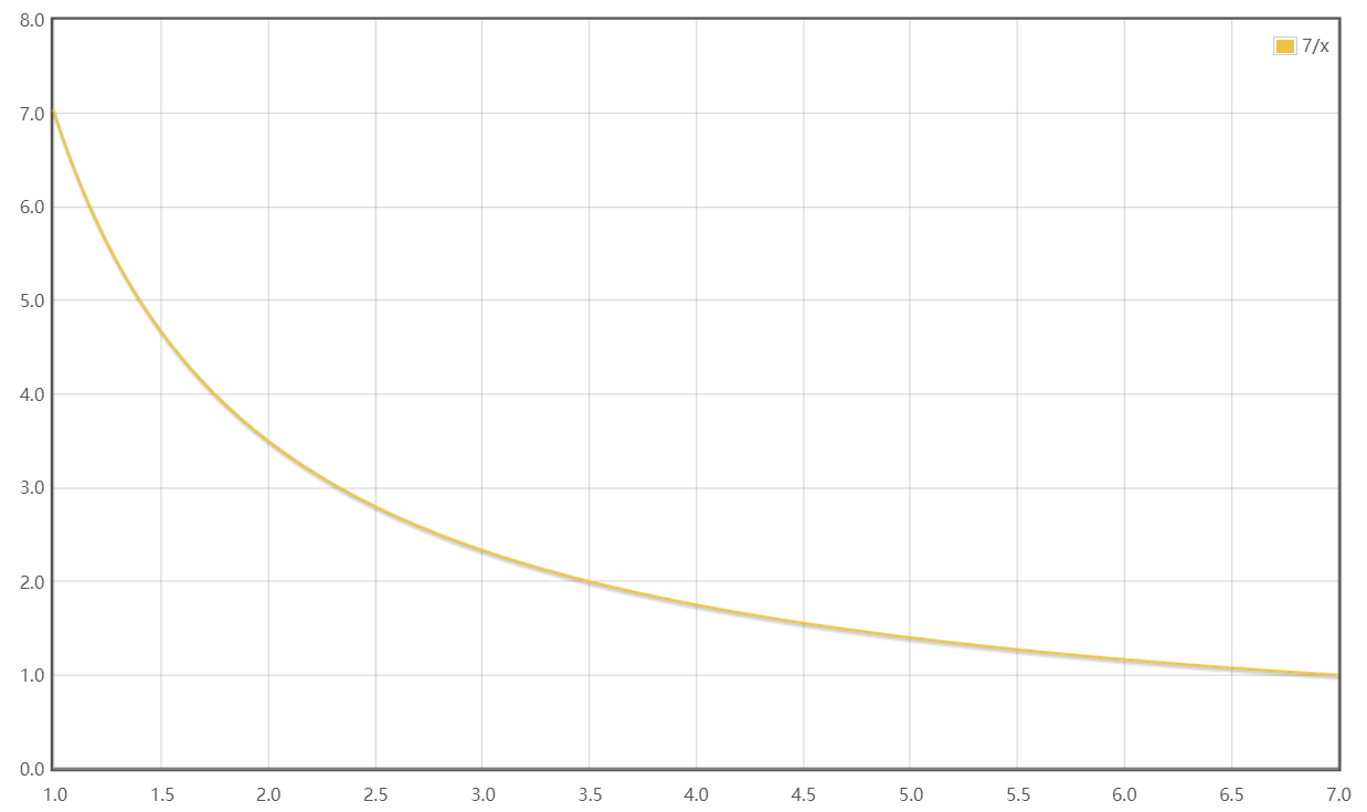
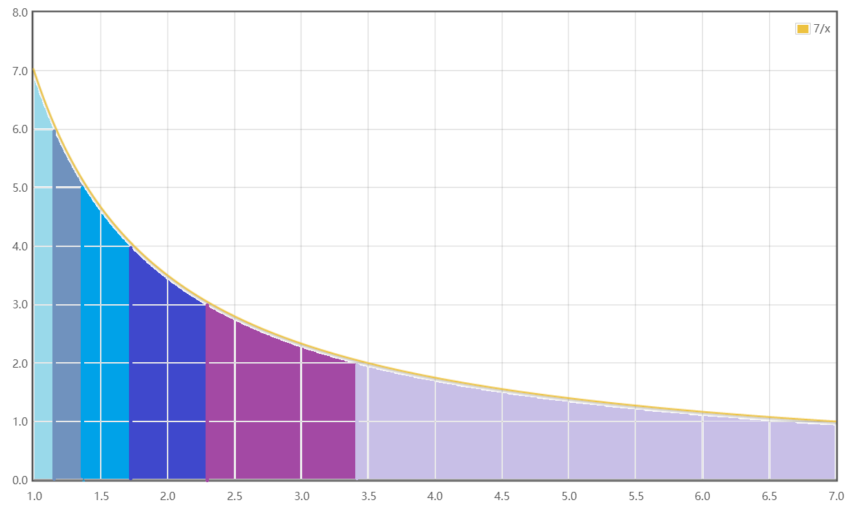
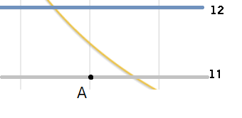
“The image splits into 7 blocks, only 4 of which contain integers. Extract the integer-containing blocks and add each block’s contribution at once.” The key fact: “for integer i, the right end of its block is $\lfloor n / \lfloor n/i \rfloor \rfloor$” — proven algebraically (squeezing $\lfloor n/\lfloor n/\lfloor n/i\rfloor\rfloor\rfloor$ between the bounds) and geometrically:
Complexity: “for $x \in [1, \lfloor\sqrt n\rfloor]$ there are at most $\lfloor\sqrt n\rfloor$ values; for $x \in (\lfloor\sqrt n\rfloor, n]$, $\lfloor n/x\rfloor$ takes at most $\lfloor\sqrt n\rfloor$ values — at most $2\lfloor\sqrt n\rfloor$ blocks, $O(\sqrt n)$.”
for (int l = 1, r; l <= x; l = r + 1)
    r = x / (x / l), res += (r - l + 1) * (x / l);
Applications: P3935 (prefix sums of divisor counts: $g(x) = \sum \lfloor x/i \rfloor$, answer $g(r)-g(l-1)$) and the sum of squared factors (blocking + square-sum formula, __int128 against overflow).
Source note: 数论分块,约数研究
7.4 Bézout’s Identity
“$ax + by = c$ has integer solutions iff $\gcd(a,b) \mid c$. Let $s = \gcd(a,b)$: $s \mid a$ and $s \mid b$, hence $s \mid ax, s \mid by$ — so c must be a multiple of the gcd.” Corollary: “two coprime numbers combine into any number.” The template answer (P4549) is simply the gcd of all inputs.
Source note: (数论)裴蜀定理
7.5 Extended Euclid and Linear Diophantine Equations
exgcd produces one particular solution of $ax + by = \gcd(a,b)$:
int exgcd(int a, int b, int &x, int &y) {
    if (!b) { x = 1, y = 0; return a; }
    int d = exgcd(b, a % b, y, x);
    y -= a / b * x;
    return d;
}
My Diophantine note completes the theory: $ax + by = c$ is solvable iff $d = \gcd(a,b) \mid c$, with infinitely many solutions $x = x_0 + \frac{b}{d}n,\ y = y_0 - \frac{a}{d}n$. Dividing through by the gcd gives $cx + dy = 1$ with $c, d$ coprime and general solution $x = x_0 + dn$, illustrated in two figures:
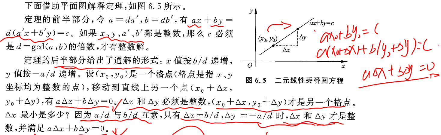
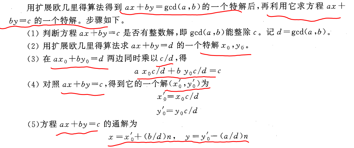
Two templates: Frog’s Date (meeting condition $(n-m)t \equiv x-y \pmod L$; smallest non-negative solution ((x*(c/d)) % (L/d) + L/d) % (L/d)) and P5656 (shift the general solution to the smallest positive x, then report solution count, max y, and the rest).
Source notes: 扩展欧几里得 解二元一次方程组 · 线性丢番图方程
7.6 Euler’s Totient, Euler’s Theorem, Fermat
$\varphi(n)$ counts integers in 1..n coprime to n. With $n = p_1^{k_1}\cdots p_m^{k_m}$, $\varphi(n) = n \prod (1 - 1/p_i)$. My proof sketch is the four-step inclusion-exclusion: “start with $n - n/p_1 - n/p_2 - \dots$; add back multiples of $p_ip_j$ (subtracted twice); subtract multiples of $p_ip_jp_k$; and so on”:

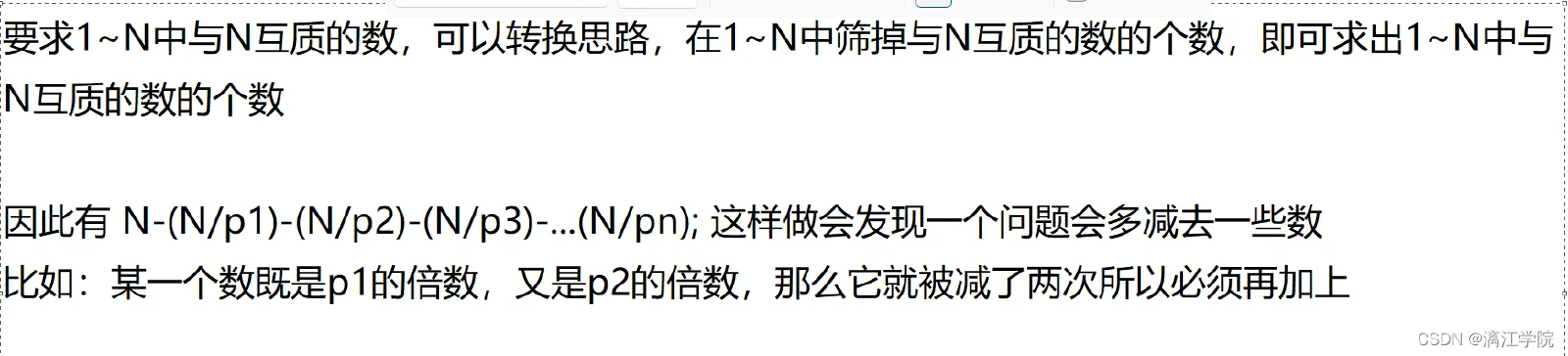
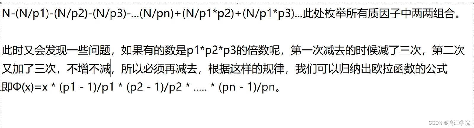
Naive evaluation writes res = res / i * (i - 1) (“same as the formula — dividing first risks floating-point trouble”); batch evaluation rides the linear sieve: when i % prime[j] == 0, $\varphi(ip) = \varphi(i)\cdot p$, else $\varphi(ip) = \varphi(i)(p-1)$. Theorems: Euler $a^{\varphi(n)} \equiv 1 \pmod n$ (gcd(a,n)=1); Fermat’s little theorem is the prime-n case $a^{n-1} \equiv 1 \pmod n$ — the theory behind computing inverses by fast power in 1.3/7.7.
Source note: 欧拉函数,欧拉定理,费马定理
7.7 Binomial Coefficients and Inclusion-Exclusion
Three tiers of $C(n,k)$ (ranges annotated in the original): $O(n^2)$ Pascal recurrence (n ≤ 2e3); factorials + Fermat inverses in $O(\log)$ (n ≤ 1e5); Lucas for huge arguments ($C(a,b) = C(a\%p, b\%p)\cdot Lucas(a/p, b/p)$). Two essential utilities: the linear inverse recurrence inv[i] = p - (p/i) * inv[p%i] % p, and backwards factorial inverses _fac[i] = _fac[i+1] * (i+1) % mod (a single fast power total).
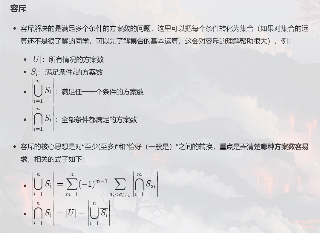
Inclusion-exclusion, from the note: “the core idea is converting between ‘at least (at most)’ and ’exactly’, through unions and intersections.”
$$\left|\bigcup_{i=1}^{n} S_i\right| = \sum_{m=1}^{n} (-1)^{m-1} \sum_{i_1 < \dots < i_m} \left|\bigcap_{j=1}^{m} S_{i_j}\right|$$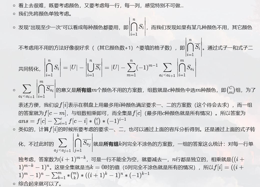
Implementation: enumerate subsets in binary (odd count adds, even subtracts; break when the product exceeds n). Two applications: Dividing Gifts (P5505 — “if i people get nothing, distribute $a_j$ gifts to n−i people: $C(a_j+n-i-1, n-i-1)$ by the insertion formula, times $C(n,i)$ for choosing them; inclusion-exclusion removes the illegal states”) and board coloring (nested exclusion over rows, columns, and colors).
7.8 Linear Basis
For “choose any subset of n numbers maximizing the XOR”. Motivation: “if the largest number has m bits, the basis shrinks $2^n$ combinations to $2^m$ — any XOR of two numbers never exceeds their highest bit, so results live in $[0, 2^m-1]$.” The example: “A = [2,3,5,6,7] has $2^n-1$ subsets but only 8 XOR results [0..7]; a basis P = [5,2,1] spans 7 of them (a basis cannot produce 0). Note: a basis is not unique.”
Construction: if every element has a distinct highest bit, A is already a basis; otherwise XOR same-length numbers together — $P = [a_1, a_1 \oplus a_2]$ spans the same set (proved by enumerating combinations in the original).
auto insert = [&](int x) -> void {
    for (int i = 61; i >= 1; i--) {
        if (x >> (i - 1)) {
            if (p[i] == 0) { p[i] = x; return; }
            else x ^= p[i];
        }
    }
    zero = true;   // a zero was formed
};
int res = 0;
for (int i = 61; i >= 1; i--) res = max(res, res ^ p[i]);Greedy correctness for the maximum: “going from high to low — for the largest, nothing else can reach its top bit; for the next, XOR it in if it helps, since any combination of smaller elements can’t beat it.” Minimum: “either 0 or the smallest-valued element.”
Source note: 线性基
7.9 Gauss-Jordan Elimination
Solve n linear equations and classify no-solution / infinite / unique. My derivation walks $2x-y+z=1$ completely: pick the largest pivot per column (“to avoid precision loss”), swap rows, normalize the pivot, zero out the rest — ending at a diagonal matrix read off directly. $O(n^3)$. Classification (“consider $ax=b$: no solution when $a=0,b\ne0$; infinite when $a=b=0$; unique when $a\ne0$. A zero pivot in some column — the largest, hence the whole column is zero — means either no solution or infinitely many”): keep a counter r (“if the pivot is 0, continue to the next column without touching r; otherwise eliminate and r←r+1. After all columns: r=n gives a unique solution; r<n means rows r+1..n are all-zero — zero right-hand sides give infinitely many, otherwise none”):
XOR systems are the key variant, with three features from my note: “when eliminating, XOR the pivot row onto the current row in reverse order; XOR systems can’t reach reduced row-echelon form — after elimination you get an upper triangle; solve from the last row upward, substituting all nonzero entries.” Each free variable doubles the answer count (on/off). Applications: Painter’s Problem (n×n tiles → influence matrix $a_{ij}$, initial colors in the constant column, free variables mean “inf”) and the switch problem (same modeling, res *= 2 per free variable).
Source note: 高斯 - 约当消元法
7.10 Matrix Exponentiation
Its purpose: “accelerating linear recurrences.” Matrix multiplication is the usual triple loop with mod; the exponentiation mirrors the numeric fast power from 1.3, with the identity matrix as the unit:
martix qpow(martix mp, int k) {
    martix res;
    for (int i = 1; i <= n; i++) res.x[i][i] = 1;   // identity
    while (k) {
        if (k & 1) res = cacl(mp, res);
        k >>= 1, mp = cacl(mp, mp);
    }
    return res;
}
Typical uses: Fibonacci-style recurrences, and counting k-step walks (the k-th power of the adjacency matrix).
Source note: 矩阵快速幂
7.11 Game Theory
Nim, via my “control” explanation: “a player with control wins — every position after his move is within his expectations. The final position is 0 0 0 0…, XOR 0. Call XOR-zero positions ‘position 0’ and the rest ‘position 1’: from position 0 the next move must go to position 1; from position 1 the player can move to position 0 — he holds control. So if the initial position is position 0, the second player wins; otherwise the first.” One line: XOR all piles; nonzero ⇒ first player wins.
High Monks Fight is the transformation example: “map it to Nim — the gaps between adjacent monks are the pile sizes, then enumerate.” Each pile is c[i] = a[i+1] - a[i] - 1; XOR odd-indexed piles to test losing positions, then enumerate moves with backtracking to find a winning one.
Source note: 博弈论
Epilogue
That’s all seven chapters. Looking back: the first note, May 2023, was about assembling sticks; the last algorithm note, November 2024, was Medium Design. In eighteen months I went from “what is KMP” to centroid decomposition and segment tree beats — every note marks a place where I got stuck and then unstuck. The cnblogs links stay here as an archive of those grinding days.
— Sakura, August 2026
Comments